使用机器学习方法预测IBM员工流失数据模型
https://www.toutiao.com/a6642158841523864067/
2019-01-03 14:50:15
在 IT公司,有许多员工架构可用。一些IT公司或特定部门或特定级别遵循主要的程序员结构,其中有一个“start”组织围绕一个“chief”职位,指定给最了解系统要求的工程师。
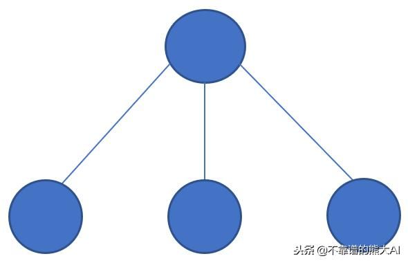
首席程序员架构
然而,有些人遵循民主结构,所有工程师都处于同一级别,指定用于不同的工作,如前端设计,后端编码,软件测试等。但是,这种架构并不是一些知名大公司所使用的。但总而言之,这是一个非常成功且有效的环境稳定型架构。
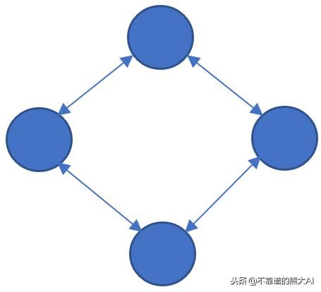
程序员民主架构
第三类架构是混合结构,它是上述两种类型的组合。这是大多数遵循的架构,在大公司中非常普遍。
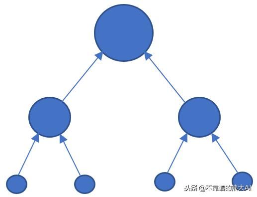
混合控制架构
同样,IBM公司可能遵循无形或混合结构。因此,对于人力资源部门来说,一项重要的责任是衡量员工在特定时间差距下的流失率。员工流失所依赖的因素是:
- 年龄
- 收入
- 加班
- 每月费用支出
- 离家的距离
- 工作年限
等等…
IBM还公开了他们的员工信息,并提供了问题陈述:
“ 预测员工的流失,即员工是否会减员,考虑到员工的详细信息,即导致员工流失的原因”
需要员工数据集的可以私信我
解决这个问题的方案是应用机器学习,通过传授机器智能涉及发展预测模型的训练,使用数据和验证模型性能分析....
以下是使用Python和Scikit-Learn机器学习工具箱进行机器学习模型开发的分步过程:
模型开发
#importing all the libraries
import numpy as np
import pandas as pd
import matplotlib.pyplot as plt
%matplotlib inline
import pylab as pl
from sklearn.metrics import roc_curve, auc
#loading the dataset using Pandas
df = pd.read_csv('WA_Fn-UseC_-HR-Employee-Attrition.csv')
df.head()# Output shown below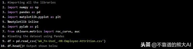
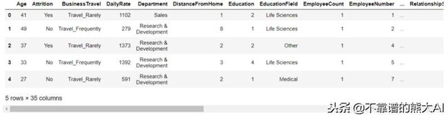
数据集的Pandas Dataframe的输出
# checking whether the dataset contains any missing values...
df.shape == df.dropna().shape # Output shown below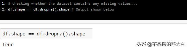
这是一个二元分类问题,因此,实例在两个类之间的分布可视化如下:
y_bar = np.array([df[df['Attrition']=='No'].shape[0]
 ,df[df['Attrition']=='Yes'].shape[0]])
x_bar = ['No (0)', 'Yes (1)'
# Bar Visualization
plt.bar(x, y)
plt.xlabel('Labels/Classes')
plt.ylabel('Number of Instances')
plt.title('Distribution of Labels/Classes in the Dataset')
# Output shown below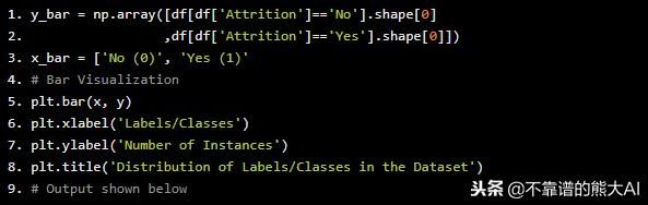
条形分布的可视化图
# Label Encoding for Categorical/Non-Numeric Data
X = df.iloc[:,[0] + list(range(2,35))].values
y = df.iloc[:,1].values
from sklearn.preprocessing import LabelEncoder, OneHotEncoder
labelencoder_X_1 = LabelEncoder()
X[:,1] = labelencoder_X_1.fit_transform(X[:,1])
X[:,3] = labelencoder_X_1.fit_transform(X[:,3])
X[:,6] = labelencoder_X_1.fit_transform(X[:,6])
X[:,10] = labelencoder_X_1.fit_transform(X[:,10])
X[:,14] = labelencoder_X_1.fit_transform(X[:,14])
X[:,16] = labelencoder_X_1.fit_transform(X[:,16])
X[:,20] = labelencoder_X_1.fit_transform(X[:,20])
X[:,21] = labelencoder_X_1.fit_transform(X[:,21])
y = labelencoder_X_1.fit_transform(y)
# Feature Selection using Random Forest Classifier's Feature
# Importance Scores
from sklearn.ensemble import RandomForestClassifier
model = RandomForestClassifier()
model.fit(X,y) # Output shown below 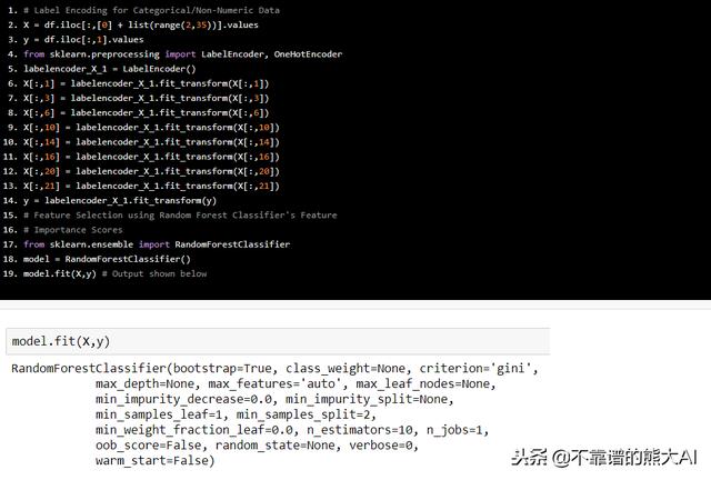
list_importances=list(model.feature_importances_)
indices=sorted(range(len(list_importances)), key=lambda k
 :list_importances[k])
feature_selected=[None]*34
k=0
for i in reversed(indices):
 if k<=33:
 feature_selected[k]=i
 k=k+1
X_selected = X[:,feature_selected[:17]]
l_features=feature_selected
i=0
for x in feature_selected:
 l_features[i] = df.columns[x]
 i=i+1
l_features = np.array(l_features)
# Extracting 17 most important features among 34 features
l_features[:17] #Output shown below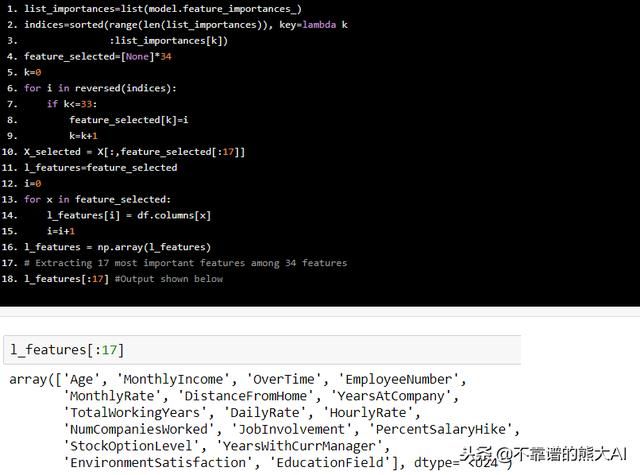
# Selecting the 17 most important features
df_features = pd.DataFrame(X_selected, columns=['Age',
'MonthlyIncome', 'OverTime',
'EmployeeNumber', 'MonthlyRate',
, 'DistanceFromHome', 'YearsAtCompany',
'TotalWorkingYears', 'DailyRate',
'HourlyRate', 'NumCompaniesWorked',
'JobInvolvement', 'PercentSalaryHike',
'StockOptionLevel',
'YearsWithCurrManager',
'EnvironmentSatisfaction',
'EducationField', 'Attrition']]
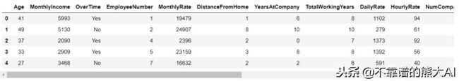
df_selected.head() # Output shown below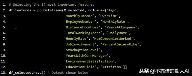
标签编码也必须对选定的分类特征进行编码:
# Label Encoding for selected Non-Numeric Features:
X = df_selected.iloc[:,list(range(0,17))].values
y = df_selected.iloc[:,17].values
X[:,2] = labelencoder_X_1.fit_transform(X[:,2])
X[:,16] = labelencoder_X_1.fit_transform(X[:,16])
y = labelencoder_X_1.fit_transform(y)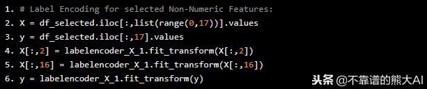
现在数据预处理已经完成。继续进行模拟训练:
# 80-20 splitting where 80% Data is for Training the Model
# and 20% Data is for Validation and Performance Analysis
from sklearn.model_selection import train_test_split
X_train, X_test, y_train, y_test = train_test_split(X, y,
 test_size=0.2, random_state=1753)
# Using Logistic Regression Algorithm for Model Training
from sklearn.linear_model import LogisticRegression
clf= LogisticRegression(verbose = 3)
# Training the Model
clf_trained = clf.fit(X_train, y_train) #Output shown below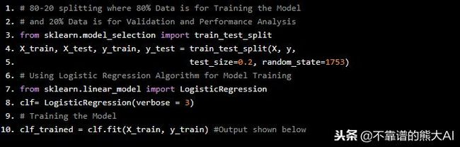
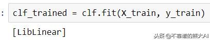
这是逻辑回归使用的参数优化策略库
2. 模型性能分析:
=> 训练准确度
clf_trained.score(X_train,y_train) # Output shown below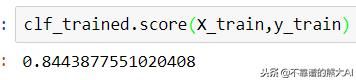
该模型的训练精度为84.44%
=> 验证准确度
clf_trained.score(X_test,y_test) # Output shown below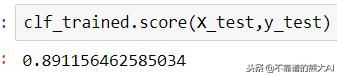
验证该模型的准确度为89.12%
=> 精确,召回率和F1-分数
# getting the predictions...
predictions=clf_trained.predict(X_test)
print(classification_report(y_test,predictions)) 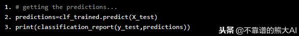

模型分类报告
=> 混淆矩阵
# MODULE FOR CONFUSION MATRIX
import matplotlib.pyplot as plt
%matplotlib inline
import numpy as np
import itertools
def plot_confusion_matrix(cm, classes,
 normalize=False,
 title='Confusion matrix',
 cmap=plt.cm.Blues):
 """
 This function prints and plots the confusion matrix.
 Normalization can be applied by setting `normalize=True`.
 """
 if normalize:
 cm = cm.astype('float') / cm.sum(axis=1)[:, np.newaxis]
 print("Normalized confusion matrix")
 else:
 print('Confusion matrix, without normalization')
print(cm)
plt.imshow(cm, interpolation='nearest', cmap=cmap)
 plt.title(title)
 plt.colorbar()
 tick_marks = np.arange(len(classes))
 plt.xticks(tick_marks, classes, rotation=45)
 plt.yticks(tick_marks, classes)
fmt = '.2f' if normalize else 'd'
 thresh = cm.max() / 2.
 for i, j in itertools.product(range(cm.shape[0])
 , range(cm.shape[1])):
 plt.text(j, i, format(cm[i, j], fmt),
 horizontalalignment="center",
 color="white" if cm[i, j] > thresh else "black")
 plt.tight_layout()
 plt.ylabel('True label')
 plt.xlabel('Predicted label')
# Generating the Confusion Matrix
plt.figure()
cm = np.array([[252, 1], [31, 10]])
plot_confusion_matrix(confusion_matrix(y_test,predictions),
 classes=[0,1], normalize=True
 , title='Normalized Confusion Matrix')
# Output shown below 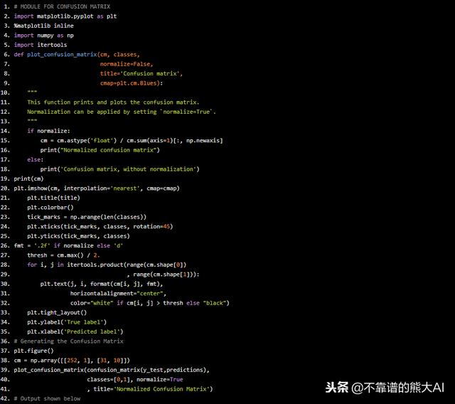
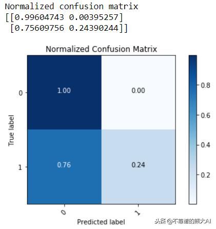
归一化混淆矩阵
=> 特征曲线:
# Plotting the ROC Curve
y_roc = np.array(y_test)
fpr, tpr, thresholds = roc_curve(y_roc, clf_trained.decision_function(X_test))
roc_auc = auc(fpr, tpr)
pl.clf()
pl.plot(fpr, tpr, label='ROC curve (area = %0.2f)' % roc_auc)
pl.plot([0, 1], [0, 1], 'k--')
pl.xlim([0.0, 1.0])
pl.ylim([0.0, 1.0])
pl.xlabel('False Positive Rate')
pl.ylabel('True Positive Rate')
pl.legend(loc="lower right")
pl.show() # Output shown below 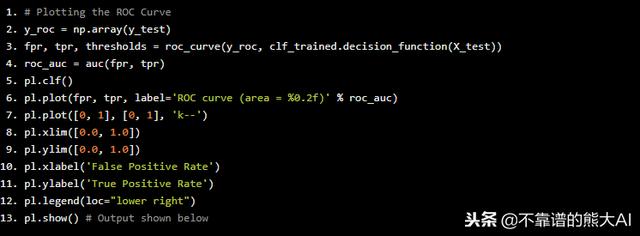

特征曲线(ROC曲线)
通过性能分析可以得出,机器学习预测模型成功地对89.12%的未知(验证集)样本进行了正确有效的分类,并对不同的性能指标给出了较低的统计数据。
因此,通过这种方式,可以使用数据分析和机器学习建立员工流失预测模型。