Intel Realsense D435深度精度测试
文章目录
-
- 数据分析:
-
- 500mm左右测量
-
- 4_1599623292.4111953.npz
-
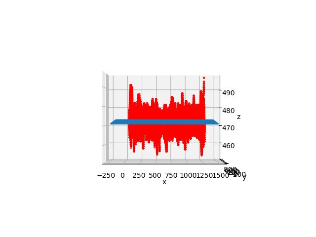
- 像素点深度及拟合平面斜视图
- 像素点深度及拟合平面正视图
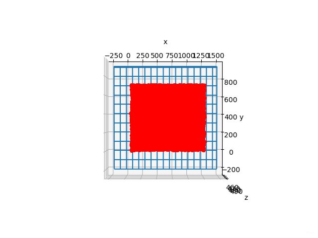
- 像素点深度及拟合平面俯视图
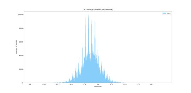
- 深度误差分布柱状图
- 深度误差分布x-y方向色彩映射图(非绝对值误差,考虑正向误差和负向误差)
- 深度误差分布x-y方向色彩映射图(非绝对值误差,考虑正向误差和负向误差)
- 代码
方法:通过采集Intel Realsense D435深度摄像头对一定深度范围内稳定平面的深度数据,去除掉黑洞及无效深度(指极端数值)后,将数据进行平面拟合,计算深度偏差,并绘制柱状图
数据分析:
500mm左右测量
4_1599623292.4111953.npz
| 文件名 | 深度分辨率 | 总点数量 | 有效点数量 | 拟合平面 |
|---|---|---|---|---|
| 4_1599623292.4111953.npz | 1280×720 | 921600 | 848866 | z = -0.000024 * x + 0.001717 * y + 471.447821 |
像素点深度及拟合平面斜视图

像素点深度及拟合平面正视图
像素点深度及拟合平面俯视图
深度误差分布柱状图
深度误差分布x-y方向色彩映射图(非绝对值误差,考虑正向误差和负向误差)
蓝色代表负向误差,绿色代表中间数值(误差小),黄色代表正向误差,红色代表越限数值和空洞

深度误差分布x-y方向色彩映射图(非绝对值误差,考虑正向误差和负向误差)

蓝色代表误差小(无论正负),绿色到黄色代表误差逐渐增加,红色代表超限或空洞
代码
- 读取并存储Intel Realsense D435摄像头深度数据
# -*- coding: utf-8 -*-
"""
@File : 摄像头精度测试.py
@Time : 2020/9/7 10:49
@Author : Dontla
@Email : [email protected]
@Software: PyCharm
"""
import datetime
import time
from datetime import date
import pyrealsense2 as rs
import cv2 as cv
import numpy as np
import matplotlib.pyplot as plt
from mpl_toolkits.mplot3d import Axes3D
from numba import jit
def cam_reset():
'''循环reset摄像头'''
# hardware_reset()后是不是应该延迟一段时间?不延迟就会报错
print('\n', end='')
print('开始初始化摄像头:')
ctx = rs.context()
for dev in ctx.query_devices():
dev.hardware_reset()
# 像下面这条语句居然不会报错,不是刚刚才重置了dev吗?莫非区别在于没有通过for循环ctx.query_devices()去访问?
# 是不是刚重置后可以通过ctx.query_devices()去查看有这个设备,但是却没有存储设备地址?如果是这样,
# 也就能够解释为啥能够通过len(ctx.query_devices())函数获取设备数量,但访问序列号等信息就会报错的原因了
time.sleep(5)
print('摄像头{}初始化成功'.format(dev.get_info(rs.camera_info.serial_number)))
def fit_flat(x, y, z):
# 取样点数量
point_num = len(x)
print(point_num)
# 创建系数矩阵A
a = 0
A = np.ones((point_num, 3))
for i in range(0, point_num):
A[i, 0] = x[a]
A[i, 1] = y[a]
a = a + 1
# print(A)
# 创建矩阵b
b = np.zeros((point_num, 1))
a = 0
for i in range(0, point_num):
b[i, 0] = z[a]
a = a + 1
# print(b)
# 通过X=(AT*A)-1*AT*b直接求解
A_T = A.T
A1 = np.dot(A_T, A)
A2 = np.linalg.inv(A1)
A3 = np.dot(A2, A_T)
X = np.dot(A3, b)
print('平面拟合结果为:z = %.3f * x + %.3f * y + %.3f' % (X[0, 0], X[1, 0], X[2, 0]))
# 计算方差
R = 0
for i in range(0, point_num):
R = R + (X[0, 0] * x[i] + X[1, 0] * y[i] + X[2, 0] - z[i]) ** 2
print('方差为:%.*f' % (3, R))
# 展示图像
fig1 = plt.figure()
ax1 = fig1.add_subplot(111, projection='3d')
ax1.set_xlabel("x")
ax1.set_ylabel("y")
ax1.set_zlabel("z")
ax1.scatter(x, y, z, c='r', marker='o')
x_p = np.linspace(0, 1500, 150)
y_p = np.linspace(0, 1500, 150)
x_p, y_p = np.meshgrid(x_p, y_p)
z_p = X[0, 0] * x_p + X[1, 0] * y_p + X[2, 0]
ax1.plot_wireframe(x_p, y_p, z_p, rstride=10, cstride=10)
plt.show()
def run_cam():
ctx = rs.context()
pipeline = rs.pipeline(ctx)
cfg = rs.config()
cfg.enable_stream(rs.stream.depth, 1280, 720, rs.format.z16, 30)
cfg.enable_stream(rs.stream.color, 1280, 720, rs.format.bgr8, 30)
profile = pipeline.start(cfg)
try:
count = 0
while True:
fs = pipeline.wait_for_frames()
# color_frame = fs.get_color_frame()
depth_frame = fs.get_depth_frame()
# print(type(depth_frame)) # - 加载深度数据并绘制相关数据图表
# -*- coding: utf-8 -*-
"""
@File    : 测试拟合平面.py
@Time    : 2020/9/8 9:23
@Author  : Dontla
@Email   : [email protected]
@Software: PyCharm
"""
import numpy as np
import matplotlib.pyplot as plt
from mpl_toolkits.mplot3d import Axes3D
from numba import jit
import cv2 as cv


# 加载数据
def load_data(file_path):
    # 读取数据
    npzfile = np.load(file_path)
    # x, y, z = npzfile['arr_0'], npzfile['arr_1'], npzfile['arr_2']
    return npzfile['x'], npzfile['y'], npzfile['z']


# 计算拟合片面
def cal_flat(x_, y_, z_):
    # 取样点数量
    point_num = len(x_)
    print('len={}'.format(point_num))

    # 创建系数矩阵A
    a = 0
    A = np.ones((point_num, 3))
    for i in range(0, point_num):
        A[i, 0] = x_[a]
        A[i, 1] = y_[a]
        a = a + 1
    # print(A)

    # 创建矩阵b
    b = np.zeros((point_num, 1))
    a = 0
    for i in range(0, point_num):
        b[i, 0] = z_[a]
        a = a + 1
    # print(b)

    # 通过X=(AT*A)-1*AT*b直接求解
    A_T = A.T
    A1 = np.dot(A_T, A)
    A2 = np.linalg.inv(A1)
    A3 = np.dot(A2, A_T)
    X = np.dot(A3, b)
    print('平面拟合结果为:z = %.6f * x + %.6f * y + %.6f' % (X[0, 0], X[1, 0], X[2, 0]))

    # 计算方差
    R = 0
    for i in range(0, point_num):
        R = R + (X[0, 0] * x_[i] + X[1, 0] * y_[i] + X[2, 0] - z_[i]) ** 2
    print('方差为:%.*f' % (3, R))
    return X


# 绘制三维深度散点图及拟合平面
def show_flat(X):
    # 展示图像
    fig1 = plt.figure()
    ax1 = fig1.add_subplot(111, projection='3d')
    ax1.set_xlabel("x")
    ax1.set_ylabel("y")
    ax1.set_zlabel("z")

    # 设定视角
    # print('ax.azim {}'.format(ax1.azim))  # -60
    # print('ax.elev {}'.format(ax1.elev))  # 30
    # 正视图
    # elev, azim = 0, -90
    # 俯视图
    # elev, azim = 90, -90

    # ax1.view_init(elev, azim)  # 设定视角

    # ax1.scatter(x, y, z, c='r', marker='o')
    ax1.scatter(x, y, z, c='r', marker='.')
    x_p = np.linspace(-200, 1480, 168)
    y_p = np.linspace(-200, 920, 112)
    x_p, y_p = np.meshgrid(x_p, y_p)
    z_p = X[0, 0] * x_p + X[1, 0] * y_p + X[2, 0]
    ax1.plot_wireframe(x_p, y_p, z_p, rstride=10, cstride=10)
    plt.show()


# 计算深度误差
def cal_error_distribution(x_, y_, z_, coefficient_):
    # 计算误差
    error = z_ - (coefficient_[0, 0] * x_ + coefficient_[1, 0] * y_ + coefficient_[2, 0])
    return error


# 统计各个区间误差的数量
def count_error_number(depth_error_, column_num):
    # 提取负向最大深度误差和正向最大深度误差
    error_max = np.max(depth_error)
    # print(error_max)    # 23.39967553034205
    error_min = np.min(depth_error)
    # print(error_min)  # -18.65760653439031

    # 柱子宽度
    error_width = (error_max - error_min) / column_num
    # print(column_width) # 1.6822912825892944

    # 创建柱子高度序列
    column_height_sequence = np.zeros(column_num)

    # 统计每个柱子包含深度点的数量
    for error in depth_error_:
        index = int((error - error_min) // error_width)
        # 当深度误差error等于最大深度误差的时候,下标会溢出,所以要加个判断限制一下
        if index == column_num:
            # print(dep)  # 23.39967553034205
            index -= 1
        column_height_sequence[index] += 1
    # print(column_height_sequence)
    return column_height_sequence


# 绘制柱状图
def draw_histogram(column_height_sequence_):
    # 创建一个点数为 8 x 6 的窗口, 并设置分辨率为 80像素/每英寸
    plt.figure(figsize=(10, 10), dpi=80)
    # plt.figure()
    # 再创建一个规格为 1 x 1 的子图
    # plt.subplot(1, 1, 1)
    # 柱子总数
    N = len(column_height_sequence)
    # 包含每个柱子对应值的序列
    values = column_height_sequence_
    # 包含每个柱子下标的序列
    index = np.arange(N)
    # 柱子的宽度
    width = 1
    # 绘制柱状图, 每根柱子的颜色为紫罗兰色
    # p2 = plt.bar(index, values, width, label="num", color="#87CEFA")
    p2 = plt.bar(index, values, width, label="num", color="#87CEFA")
    # 设置横轴标签
    plt.xlabel('error/mm')
    # 设置纵轴标签
    plt.ylabel('number of points')
    # 添加标题
    plt.title('D435 error Distribution(500mm)')
    # 添加纵横轴的刻度
    index_new = []
    for index_ in index:
        if index_ % 100 == 0:
            index_new.append(index_)
    # print(index_new)
    index_new_content = []
    for index in index_new:
        error_max = np.max(depth_error)
        error_min = np.min(depth_error)
        index_new_content.append(error_min + (error_max - error_min) * index / N)
    index_new_content_string = [str(i) for i in np.around(index_new_content, decimals=1)]
    # plt.xticks(index, (
    #     'mentioned1cluster', 'mentioned2cluster', 'mentioned3cluster', 'mentioned4cluster', 'mentioned5cluster',
    #     'mentioned6cluster', 'mentioned7cluster', 'mentioned8cluster', 'mentioned9cluster', 'mentioned10cluster'))
    plt.xticks(index_new, index_new_content_string)
    # plt.yticks(np.arange(0, 10000, 10))
    # 添加图例
    plt.legend(loc="upper right")
    plt.show()


# 使用opencv绘制误差x-y方向(非绝对值)分布图
def draw_tangential_distribution_opencv(x_, y_, depth_error_):
    error_max2min = np.max(depth_error_) - np.min(depth_error_)
    error_array = np.ones((720, 1280)) * error_max2min
    error_min = np.min(depth_error_)
    for i in range(len(x_)):
        error_array[y_[i], x_[i]] = depth_error_[i] - error_min  # 全转换为正的,好画图
    alp = 255 / error_max2min
    error_image = cv.applyColorMap(cv.convertScaleAbs(error_array, alpha=alp), cv.COLORMAP_JET)
    cv.imshow('window', error_image)
    cv.waitKey(0)


# 使用opencv绘制误差x-y方向(绝对值)分布图
def draw_tangential_distribution_opencv_abs(x_, y_, depth_error_):
    error_max2min = np.max(depth_error_) - np.min(depth_error_)
    error_array = np.ones((720, 1280)) * error_max2min
    for i in range(len(x_)):
        error_array[y_[i], x_[i]] = depth_error_[i]
    error_array_abs = np.abs(error_array)
    max_abs = np.maximum(np.abs(np.min(depth_error_)), np.abs(np.max(depth_error_)))
    alp = 255 / max_abs
    error_image = cv.applyColorMap(cv.convertScaleAbs(error_array_abs, alpha=alp), cv.COLORMAP_JET)
    cv.imshow('window', error_image)
    cv.waitKey(0)


if __name__ == '__main__':
    # 加载数据
    x, y, z = load_data('./data/1000mm/4_1599635389.3573992.npz')

    # 拟合平面并返回平面函数系数
    coefficient = cal_flat(x, y, z)

    # 绘制平面及深度散点
    show_flat(coefficient)

    # 计算深度误差
    depth_error = cal_error_distribution(x, y, z, coefficient)

    # 统计各个误差区间的数量(柱状图各个柱子高度)
    column_height_sequence = count_error_number(depth_error, 1000)

    # 绘制柱状图
    draw_histogram(column_height_sequence)

    # 用opencv绘制误差x-y方向分布图(非绝对值)
    draw_tangential_distribution_opencv(x, y, depth_error)

    # 用opencv绘制误差x-y方向分布图(绝对值)
    draw_tangential_distribution_opencv_abs(x, y, depth_error)

