机器学习系列4---RVM（相关向量机）MATLAB实现

       上期主要介绍了相关向量机的提出及主要计算过程，本期主要介绍MATLAB实现RVM，并就相关分析结果展开讨论。相关论文及代码下载网站：http://www.miketipping.com/sparsebayes.htm；RVM分为定量和定性分析两种类型，首先介绍定量分析：定量分析通过随机产sinc函数数据点进行稀疏表示学习，然后将拟合结果和真实数据进行对比，计算RMSE判定分析性能。

1.RVM定量分析MATLAB代码

%% Set verbosity of output (0 to 4)
setEnvironment('Diagnostic','verbosity',3);
% Set file ID to write to (1 = stdout)
setEnvironment('Diagnostic','fid',1);

%% 设置模型和数据参数
useBias	= true;
randn('state',1)
if nargin==0
  N		= 100;
  noise		= 0.1;
  kernel_	= 'gauss';
  width		= 3;
  maxIts	= 1200;
end
monIts		= round(maxIts/10);

%% 产生sinc数据
x	= 10*[-1:2/(N-1):1]';
y	= sin(abs(x))./abs(x);
t	= y + noise*randn(N,1);

%% 设置绘图参数
COL_data	= 'k';
COL_sinc	= 'g';
% COL_sinc	= 0.5*ones(1,3);
COL_rv		= 'r';
COL_pred	= 'r';

% 绘制sinc数据
figure(1)
whitebg(1,'w')
clf
h_y = plot(x,y,'--','LineWidth',3,'Color',COL_sinc);
hold on
plot(x,t,'.','MarkerSize',16,'Color',COL_data)
box = [-10.1 10.1 1.1*[min(t) max(t)]];
axis(box)
set(gca,'FontSize',12)
drawnow

%% 设置超参数初始值 
initAlpha	= (1/N)^2;
epsilon		= std(t) * 10/100; % Initial guess of 10% noise-to-signal
initBeta	= 1/epsilon^2;

%% 产生RVM 模型
 
[weights, used, bias, marginal, alpha, beta, gamma] = ...
    SB1_RVM(x,t,initAlpha,initBeta,kernel_,width,useBias,maxIts,monIts);

%% 模型测试
PHI	= SB1_KernelFunction(x,x,kernel_,width);
y_rvm	= PHI(:,used)*weights + bias;

%% 对比分析结果
h_yrvm	= plot(x,y_rvm,'-','LineWidth',3,'Color',COL_pred);
h_rv	= plot(x(used),t(used),'o','LineWidth',2,'MarkerSize',10,...
	       'Color',COL_rv);
legend([h_y h_yrvm h_rv],'sinc function','RVM predictor','RVs')
hold off
title('Sparse Bayesian regression with noisy ''sinc'' data','FontSize',14)

SB1_Diagnostic(1,'Sparse Bayesian regression test error (RMS): %g\n', ...
	sqrt(mean((y-y_rvm).^2)))
SB1_Diagnostic(1,'Estimated noise level: %.4f (true: %.4f)\n', ...
	sqrt(1/beta), noise)

2. RVM定量分析结果

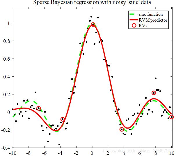
超参数分析结果:

1.非零参数: 6 (全部:100)；

2.似然函数最小最大值:  -0.13/1.91；

3.RMSE: 0.0424557；

4.噪声估计: 0.0933 (真实值: 0.1000)。

 

3. RVM定性分析MATLAB代码

% The MATLAB demo for RVMclassificaion
% first version: 2020/5/01
clc;clear;
%%
% Set verbosity of output (0 to 4)
setEnvironment('Diagnostic','verbosity',3);
% Set file ID to write to (1 = stdout)
setEnvironment('Diagnostic','fid',1);

%% Set default values for data and model
useBias	= true;
rand('state',1)
% Some acceptable defaults
N		= 100;
kernel_	= 'gauss';
width		= 0.5;
maxIts	= 1000;
monIts		= round(maxIts/10);
N		= min([250 N]); % training set has fixed size of 250
Nt		= 1000;
%% Load Ripley's synthetic training data (see reference in doc)
load synth.tr
synth	= synth(randperm(size(synth,1)),:);
X	= synth(1:N,1:2);
t	= synth(1:N,3);
%%
COL_data1	= 'k';
COL_data2	= 0.75*[0 1 0];
COL_boundary50	= 'r';
COL_boundary75	= 0.5*ones(1,3);
COL_rv		= 'r';
% Plot the training data 
figure(1)
whitebg(1,'w')
clf
h_c1	= plot(X(t==0,1),X(t==0,2),'.','MarkerSize',18,'Color',COL_data1);
hold on
h_c2	= plot(X(t==1,1),X(t==1,2),'.','MarkerSize',18,'Color',COL_data2);
box	= 1.1*[min(X(:,1)) max(X(:,1)) min(X(:,2)) max(X(:,2))];
axis(box)
set(gca,'FontSize',12)
drawnow
%% Set up initial hyperparameters - precise settings should not be critical
initAlpha	= (1/N)^2;
% Set beta to zero for classification
initBeta	= 0;	
% "Train" a sparse Bayes kernel-based model (relevance vector machine) 
[weights, used, bias, marginal, alpha, beta, gamma] = ...
    SB1_RVM(X,t,initAlpha,initBeta,kernel_,width,useBias,maxIts,monIts);
%% Load Ripley's test set 
load synth.te
synth	= synth(randperm(size(synth,1)),:);
Xtest	= synth(1:Nt,1:2);
ttest	= synth(1:Nt,3);
%% Compute RVM over test data and calculate error 
PHI	= SB1_KernelFunction(Xtest,X(used,:),kernel_,width);
y_rvm	= PHI*weights + bias;
errs	= sum(y_rvm(ttest==0)>0) + sum(y_rvm(ttest==1)<=0);
SB1_Diagnostic(1,'RVM CLASSIFICATION test error: %.2f%%\n', errs/Nt*100)
%% Visualise the results over a grid
gsteps		= 50;
range1		= box(1):(box(2)-box(1))/(gsteps-1):box(2);
range2		= box(3):(box(4)-box(3))/(gsteps-1):box(4);
[grid1 grid2]	= meshgrid(range1,range2);
Xgrid		= [grid1(:) grid2(:)];
%% Evaluate RVM 
PHI		= SB1_KernelFunction(Xgrid,X(used,:),kernel_,width);
y_grid		= PHI*weights + bias;
% apply sigmoid for probabilities
p_grid		= 1./(1+exp(-y_grid)); 
% Show decision boundary (p=0.5) and illustrate p=0.25 and 0.75
[c,h05]		= ...
    contour(range1,range2,reshape(p_grid,size(grid1)),[0.5],'-');
set(h05, 'Color',COL_boundary50,'LineWidth',3);
[c,h075]	= ...
    contour(range1,range2,reshape(p_grid,size(grid1)),[0.25 0.75],'--');
set(h075,'Color',COL_boundary75,'LineWidth',2);

% Show relevance vectors
h_rv	= plot(X(used,1),X(used,2),'o','LineWidth',2,'MarkerSize',10,...
	       'Color',COL_rv);
legend([h_c1 h_c2 h05 h075(1) h_rv],...
       'Class 1','Class 2','Decision boundary','p=0.25/0.75','RVs',...
       'Location','NorthWest')
hold off
title('RVM Classification of Ripley''s synthetic data','FontSize',14)

4. RVM定性分析结果

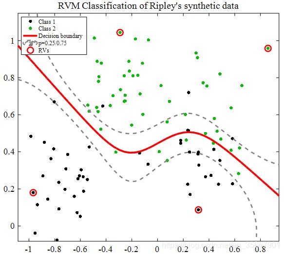
分析结果:

1.非零变量:  4；

2.似然函数最小最大值:  -1.86/-0.99；

3.RVM 分类错误率: 8.60%。

       通过上面的例子可以实现简单的RVM分析，具体的实际分析例子会后续更新。

写于2020.5.1

加油。