数据分析36计(21)：Uber、Netflix 常用倍差法模型量化营销活动、产品改版影响效果

1 案例背景

目前 Uber、Netflix 在商业分析中的因果推断常用模型主要是倍差法(Difference in Difference)和匹配（Matching），目前已在其平台中建立相关方法的自主分析工具。这篇文章将介绍倍差法和普通回归法在效应量评估上的真实差异。

这里以一个简单的经济学案例来讲述倍差法 DID 的原理，根据美国联邦法规，每个州的劳工赔偿计划在赔偿受伤的工人时，其赔偿范围从一定的“补偿率”（通常是受伤前工资的三分之二）到某个特定的最高额。对理性决策者而言，继续伤残所能获得的补偿越高，重返工作的动力就越小。

1980年，肯塔基州提高了每周工伤赔偿的最高限额，这里检验赔偿额的变化是否对重返工作的决策有显著影响。我们关心的主要结果变量是 log_duration（在数据中为 ldurat ），或记录的工伤补偿期限（以周为单位）。这里该变量取 log 是因为该变量存在较大的偏差，大多数人失业了几周，而有些人失业了很长时间。制定该政策的目的是使上限增加不会影响低收入工人，但会影响高收入工人，因此我们将低收入工人作为我们的对照组，将高收入工人作为我们的处理组。

数据集包含在 wooldridge R 软件包中的 injury：

• durat（duration）：失业救济金的持续时间，以周为单位
• ldurat（log_duration）：log(durat)
• after_1980（after_1980）：指标变量，观察是在1980年政策更改之前（0）还是之后（1）进行，时间变量：before/after
• highearn：指示变量，用于标记观察值是低（0）还是高（1）收入，分组变量：处理/对照

2 加载和清理数据

首先下载数据集并加载相关库：

library(tidyverse)  # ggplot(), %>%, mutate(), and friends
library(broom)  # Convert models to data frames
library(scales)  # Format numbers with functions like comma(), percent(), and dollar()
library(modelsummary)  # Create side-by-side regression tables

# Load the data. 
# It'd be a good idea to click on the "injury_raw" object in the Environment
# panel in RStudio to see what the data looks like after you load it
injury_raw <- read_csv("data/injury.csv")

injury <- injury_raw %>% 
  filter(ky == 1) %>% 
  # The syntax for rename is `new_name = original_name`
  rename(duration = durat, log_duration = ldurat,
         after_1980 = afchnge)

3 探索性数据分析

首先可以看看高低收入者（对照和处理组）中失业补偿的分布：

ggplot(data = injury, aes(x = duration)) +
  # binwidth = 8 makes each column represent 2 months (8 weeks) 
  # boundary = 0 make it so the 0-8 bar starts at 0 and isn't -4 to 4
  geom_histogram(binwidth = 8, color = "white", boundary = 0) +
  facet_wrap(vars(highearn))

分配情况确实存在偏差，两组中的大多数人都可以享受 0-8 周的福利（还有少数可以享受 180 周以上的福利！这就是 3.5 年！）

如果使用持续时间的对数，则可以得到较少偏斜的分布，该分布更适合回归模型：

ggplot(data = injury, mapping = aes(x = log_duration)) +
  geom_histogram(binwidth = 0.5, color = "white", boundary = 0) + 
  # Uncomment this line if you want to exponentiate the logged values on the
  # x-axis. Instead of showing 1, 2, 3, etc., it'll show e^1, e^2, e^3, etc. and
  # make the labels more human readable
  # scale_x_continuous(labels = trans_format("exp", format = round)) +
  facet_wrap(vars(highearn))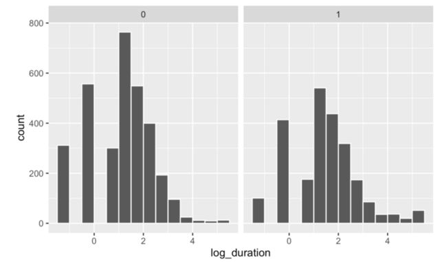

我们还应该检查政策改变前后的失业情况：

ggplot(data = injury, mapping = aes(x = log_duration)) +
  geom_histogram(binwidth = 0.5, color = "white", boundary = 0) + 
  facet_wrap(vars(after_1980))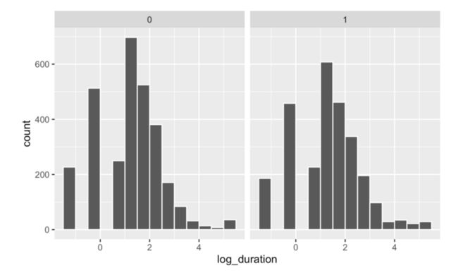

分布看上去很正常，但很难轻易看出处理前后，即对照组与处理组之间的差异。我们可以绘制平均值。使用 stat_summary() 图层让 ggplot 计算汇总平均值等汇总统计信息。这里我们只计算平均值：

ggplot(injury, aes(x = factor(highearn), y = log_duration)) +
  geom_point(size = 0.5, alpha = 0.2) +
  stat_summary(geom = "point", fun = "mean", size = 5, color = "red") +
  facet_wrap(vars(after_1980))

计算平均值和 95％ 置信区间：

ggplot(injury, aes(x = factor(highearn), y = log_duration)) +
  stat_summary(geom = "pointrange", size = 1, color = "red",
               fun.data = "mean_se", fun.args = list(mult = 1.96)) +
  facet_wrap(vars(after_1980))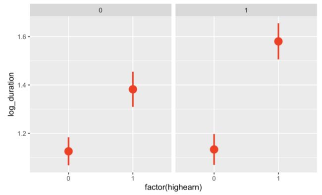

可以开始看到经典的差异比较图！看起来 1980 年以后的高收入者平均失业时间更长。在将数据发送到 ggplot 之前，还可以使用 group_by() 和 summarize() 找出分组均值：

ggplot(plot_data, aes(x = after_1980, y = mean_duration, color = highearn)) +
  geom_pointrange(aes(ymin = lower, ymax = upper), size = 1) + 
  # The group = highearn here makes it so the lines go across categories
  geom_line(aes(group = highearn))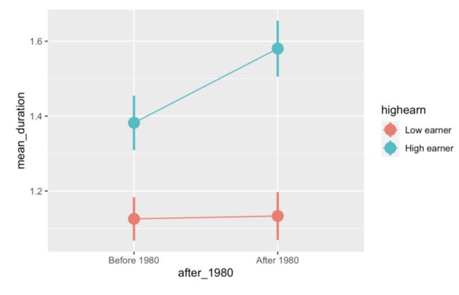

4 倍差法 DID 的计算原理

我们可以通过填写 2x2 来找到对照组和处理组间的真实差异：

diffs <- injury %>% 
  group_by(after_1980, highearn) %>% 
  summarize(mean_duration = mean(log_duration),
    # Calculate average with regular duration too, just for fun
    mean_duration_for_humans = mean(duration))
diffs

## # A tibble: 4 x 4
## # Groups:   after_1980 [2]
##   after_1980 highearn mean_duration mean_duration_for_humans
##                                         
## 1          0        0          1.13                     6.27
## 2          0        1          1.38                    11.2 
## 3          1        0          1.13                     7.04
## 4          1        1          1.58                    12.9

before_treatment <- diffs %>% 
  filter(after_1980 == 0, highearn == 1) %>% 
  pull(mean_duration)

before_control <- diffs %>% 
  filter(after_1980 == 0, highearn == 0) %>% 
  pull(mean_duration)

after_treatment <- diffs %>% 
  filter(after_1980 == 1, highearn == 1) %>% 
  pull(mean_duration)

after_control <- diffs %>% 
  filter(after_1980 == 1, highearn == 0) %>% 
  pull(mean_duration)

diff_treatment_before_after <- after_treatment - before_treatment
diff_control_before_after <- after_control - before_control
diff_diff <- diff_treatment_before_after - diff_control_before_after
diff_diff
## 0.19

对照组和处理组的差异估计为 0.19，这意味着该政策计划导致失业时间增加 19％。

5 倍差法 DID 回归

像上面的手工计算很繁琐，因此我们可以使用回归来完成！请记住，我们需要包括用于处理/对照组、1980前/后以及两者之间交互作用的指标变量：
系数是我们最终关心的效果，即 DID 估计量。

model_small <- lm(log_duration ~ highearn + after_1980 + highearn * after_1980,data = injury)
tidy(model_small)

## # A tibble: 4 x 5
##   term                estimate std.error statistic   p.value
##                                    
## 1 (Intercept)          1.13       0.0307    36.6   1.62e-263
## 2 highearn             0.256      0.0474     5.41  6.72e-8
## 3 after_1980           0.00766    0.0447     0.171 8.64e-1
## 4 highearn:after_1980  0.191      0.0685     2.78  5.42e-3

highearn:after_1980 的系数应该与我们手动计算的系数相同！它具有统计意义，因此我们可以确信高低收入之间的失业时长存在显著差异。

6 加入控制变量的 DID 回归

DID 回归的优点之一是，可以包括控制变量。例如，与其他行业的工人相比，建筑或制造业工人的工人索赔期限往往更长。我们可能还希望控制工人的人口统计信息，例如性别，婚姻状况和年龄。

让我们用以下附加变量估算基本回归模型：

• male
• married
• age
• hosp （1=住院）
• indust （1=制造商，2=建筑，3=其他）
• injtype （1-8；不同类型伤害的类别）
• lprewage （提出索赔之前的工资记录）

提示：indust 和 injtype 在数据集中以数字（1-3和1-8）表示，但实际上它们是类别。在 R 中必须将它们视为类别（或因子）。

# Convert industry and injury type to categories/factors
injury_fixed <- injury %>% 
  mutate(indust = as.factor(indust),
         injtype = as.factor(injtype))
         
model_big <- lm(log_duration ~ highearn + after_1980 + highearn * after_1980 + 
                  male + married + age + hosp + indust + injtype + lprewage,
                data = injury_fixed)
tidy(model_big)

# Extract just the diff-in-diff estimate
diff_diff_controls <- tidy(model_big) %>% 
  filter(term == "highearn:after_1980") %>% 
  pull(estimate)
  
modelsummary(list("DID" = model_small, "DID+control" = model_big))

	DID	DID+control
(Intercept)	1.126***	-1.528***
	(0.031)	(0.422)
highearn	0.256***	-0.152*
	(0.047)	(0.089)
after\_1980	0.008	0.050
	(0.045)	(0.041)
highearn × after\_1980	0.191***	0.169***
	(0.069)	(0.064)
male		-0.084**
		(0.042)
married		0.057
		(0.037)
age		0.007***
		(0.001)
hosp		1.130***
		(0.037)
indust2		0.184***
		(0.054)
indust3		0.163***
		(0.038)
injtype2		0.935***
		(0.144)
injtype3		0.635***
		(0.085)
injtype4		0.555***
		(0.093)
injtype5		0.641***
		(0.085)
injtype6		0.615***
		(0.086)
injtype7		0.991***
		(0.191)
injtype8		0.434***
		(0.119)
lprewage		0.284***
		(0.080)
Num.Obs.	5626	5347
R2	0.021	0.190
R2 Adj.	0.020	0.187

* p \< 0.1, ** p \< 0.05, *** p \< 0.01

在控制了许多人口统计因素之后，“差异比较”估计值变小（0.169），表明该政策导致工作场所受伤后的失业时间延长了16.9％。之所以较小，是因为其他自变量可以解释的部分log_duration的变化。

其余文章阅读请移步公众h：DataGo数据狗

本文由博客群发一文多发等运营工具平台 OpenWrite 发布