学术前沿趋势分析

TASK1

任务说明

任务主题：论文数量统计，即统计2019年全年计算机各个方向论文数量；
任务内容：赛题的理解、使用 Pandas 读取数据并进行统计；
任务成果：学习 Pandas 的基础操作；
可参考的学习资料：开源组织Datawhale joyful-pandas项目

数据集介绍

数据集的格式如下：
id：arXiv ID，可用于访问论文；
submitter：论文提交者；
authors：论文作者；
title：论文标题；
comments：论文页数和图表等其他信息；
journal-ref：论文发表的期刊的信息；
doi：数字对象标识符，https://www.doi.org；
report-no：报告编号；
categories：论文在 arXiv 系统的所属类别或标签；
license：文章的许可证；
abstract：论文摘要；
versions：论文版本；
authors_parsed：作者的信息。

“root”:{
“id”:string"0704.0001"
“submitter”:string"Pavel Nadolsky"
“authors”:string"C. Bal’azs, E. L. Berger, P. M. Nadolsky, C.-P. Yuan"
“title”:string"Calculation of prompt diphoton production cross sections at Tevatron and LHC energies"
“comments”:string"37 pages, 15 figures; published version"
“journal-ref”:string"Phys.Rev.D76:013009,2007"
“doi”:string"10.1103/PhysRevD.76.013009"
“report-no”:string"ANL-HEP-PR-07-12"
“categories”:string"hep-ph"
“license”:NULL
“abstract”:string" A fully differential calculation in perturbative quantum chromodynamics is presented for the production of massive photon pairs at hadron colliders. All next-to-leading order perturbative contributions from quark-antiquark, gluon-(anti)quark, and gluon-gluon subprocesses are included, as well as all-orders resummation of initial-state gluon radiation valid at next-to-next-to leading logarithmic accuracy. The region of phase space is specified in which the calculation is most reliable. Good agreement is demonstrated with data from the Fermilab Tevatron, and predictions are made for more detailed tests with CDF and DO data. Predictions are shown for distributions of diphoton pairs produced at the energy of the Large Hadron Collider (LHC). Distributions of the diphoton pairs from the decay of a Higgs boson are contrasted with those produced from QCD processes at the LHC, showing that enhanced sensitivity to the signal can be obtained with judicious selection of events."
“versions”:[
0:{
“version”:string"v1"
“created”:string"Mon, 2 Apr 2007 19:18:42 GMT"
}
1:{
“version”:string"v2"
“created”:string"Tue, 24 Jul 2007 20:10:27 GMT"
}]
“update_date”:string"2008-11-26"
“authors_parsed”:[
0:[
0:string"Balázs"
1:string"C."
2:string""]
1:[
0:string"Berger"
1:string"E. L."
2:string""]
2:[
0:string"Nadolsky"
1:string"P. M."
2:string""]
3:[
0:string"Yuan"
1:string"C. -P."
2:string""]]
}

arxiv论文类别介绍

我们从arxiv官网，查询到论文的类别名称以及其解释如下。
链接：https://arxiv.org/help/api/user-manual
的 5.3 小节的 Subject Classifications 的部分，或
https://arxiv.org/category_taxonomy，
具体的153种paper的类别部分如下：

‘astro-ph’: ‘Astrophysics’
‘astro-ph.CO’: ‘Cosmology and Nongalactic Astrophysics’
‘astro-ph.EP’: ‘Earth and Planetary Astrophysics’
‘astro-ph.GA’: ‘Astrophysics of Galaxies’
‘cs.AI’: ‘Artificial Intelligence’
‘cs.AR’: ‘Hardware Architecture’
‘cs.CC’:‘Computational Complexity’
‘cs.CE’: ‘Computational Engineering,Finance, and Science’
‘cs.CV’: ‘Computer Vision and Pattern Recognition’
‘cs.CY’: ‘Computers and Society’
‘cs.DB’: ‘Databases’
‘cs.DC’: ‘Distributed, Parallel, and Cluster Computing’
‘cs.DL’: ‘Digital Libraries’
‘cs.NA’: ‘Numerical Analysis’
‘cs.NE’: ‘Neural and Evolutionary Computing’
‘cs.NI’: ‘Networking and Internet Architecture’
‘cs.OH’: ‘Other Computer Science’
‘cs.OS’: ‘Operating Systems’

**具体代码实现以及讲解

#导入package并读取原始数据**
import seaborn as sns #用于画图
from bs4 import BeautifulSoup #用于爬取arxiv的数据
import re #用于正则表达式，匹配字符串的模式
import requests #用于网络连接，发送网络请求，使用域名获取对应信息
import json #读取数据，我们的数据为json格式的
import pandas as pd #数据处理，数据分析
import matplotlib.pyplot as plt #画图工具
# 读入数据
data  = []

#使用with语句优势：1.自动关闭文件句柄；2.自动显示（处理）文件读取数据异常
with open("arxiv-metadata-oai-snapshot.json", 'r') as f: 
    for idx, line in enumerate(f): 
        
        # 读取前100行，如果读取所有数据需要8G内存
        if idx >= 100:
            break
        
        data.append(json.loads(line))
        
data = pd.DataFrame(data) #将list变为dataframe格式，方便使用pandas进行分析
data.shape #显示数据大小
data.head(2)

(100, 14)

def readArxivFile(path,columns=['id', 'submitter', 'authors', 'title', 'comments', 'journal-ref', 'doi',
       'report-no', 'categories', 'license', 'abstract', 'versions',
       'update_date', 'authors_parsed'],count=None):
    '''
    定义读取文件的函数
        path: 文件路径
        columns: 需要选择的列
        count: 读取行数
    '''
    data=[]
    with open(path,'r') as f:
        for idx,line in enumerate(f):
            if idx==count:
                break
            d=json.loads(line)#d为字典
            d={
     col:d[col] for col in columns}
            data.append(d)
    data=pd.DataFrame(data)
    return data
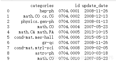
data=readArxivFile('arxiv-metadata-oai-snapshot.json', ['id', 'categories', 'update_date'])
print(data.head(10)) 
       

:

数据预处理
首先我们先来粗略统计论文的种类信息：

count：一列数据的元素个数；
unique：一列数据中元素的种类；
top：一列数据中出现频率最高的元素；
freq：一列数据中出现频率最高的元素的个数；

unique_categories=set([i for l in [x.split(' ') for x in data["categories"]] for i in l])
  
#我们的任务要求对于2019年以后的paper进行分析，所以首先对于时间特征进行预处理，从而得到2019年以后的所有种类的论文：
data['year']=pd.to_datetime(data["update_date"]).dt.year
del data["update_date"]
data=data[data['year']>=2019]
data.reset_index(drop=True,inplace=True)#重新编号
print(data.head()) 

#爬取所有的类别
# website_url=requests.get("https://arxiv.org/category_taxonomy").text
# print(website_url)
soup=BeautifulSoup(website_url,'lxml')#获取arxiv的数据，这里使用lxml的解析器，加速
# print(soup)
root=soup.find('div',{
     'id':'category_taxonomy_list'})#找出 BeautifulSoup 对应的标签入口
# print(root)
tags=root.find_all(["h2","h3","h4","p"], recursive=True) #读取 tags
#初始化 str 和 list 变量
level_1_name = ""
level_2_name = ""
level_2_code = ""
level_1_names = []
level_2_codes = []
level_2_names = []
level_3_codes = []
level_3_names = []
level_3_notes = []

for t in tags:
    if t.name == "h2":
        level_1_name = t.text    
        level_2_code = t.text
        level_2_name = t.text
    elif t.name == "h3":
        raw = t.text
        level_2_code = re.sub(r"(.*)\((.*)\)",r"\2",raw) #正则表达式：模式字符串：(.*)\((.*)\)；被替换字符串"\2"；被处理字符串：raw
        level_2_name = re.sub(r"(.*)\((.*)\)",r"\1",raw)
    elif t.name == "h4":
        raw = t.text
        level_3_code = re.sub(r"(.*) \((.*)\)",r"\1",raw)
        level_3_name = re.sub(r"(.*) \((.*)\)",r"\2",raw)
    elif t.name == "p":
        notes = t.text
        level_1_names.append(level_1_name)
        level_2_names.append(level_2_name)
        level_2_codes.append(level_2_code)
        level_3_names.append(level_3_name)
        level_3_codes.append(level_3_code)
        level_3_notes.append(notes)
        
#根据以上信息生成dataframe格式的数据
df_taxonomy = pd.DataFrame({
     
    'group_name' : level_1_names,
    'archive_name' : level_2_names,
    'archive_id' : level_2_codes,
    'category_name' : level_3_names,
    'categories' : level_3_codes,
    'category_description': level_3_notes
    
})

#按照 "group_name" 进行分组，在组内使用 "archive_name" 进行排序
df_taxonomy.groupby(["group_name","archive_name"])

数据分析及可视化

接下来我们首先看一下所有大类的paper数量分布：

我们使用merge函数，以两个dataframe共同的属性 “categories” 进行合并，并以 “group_name”
作为类别进行统计，统计结果放入 “id” 列中并排序。

_df = data.merge(df_taxonomy, on="categories", how="left").drop_duplicates(["id","group_name"]).groupby("group_name").agg({
     "id":"count"}).sort_values(by="id",ascending=False).reset_index() 
_df

group_name	id
Physics	79985
Mathematics	51567
Computer Science	40067
Statistics	4054
Electrical Engineering and Systems Science	3297
Quantitative Biology	1994
Quantitative Finance	826
Economics	576

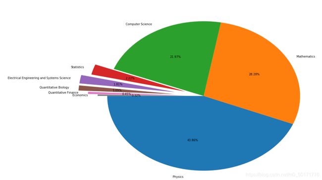
下面我们使用饼图进行上图结果的可视化：

fig = plt.figure(figsize=(15,12))
explode = (0, 0, 0, 0.2, 0.3, 0.3, 0.2, 0.1)#分开
# explode = (0.2, 0.2, 0.2, 0.2, 0.3, 0.3, 0.2, 0.1)
plt.pie(_df["id"],  labels=_df["group_name"], autopct='%1.2f%%',explode=explode,startangle=180)#startangle=180旋转角度
# plt.tight_layout()#tight_layout会自动调整子图参数
plt.show()

下面统计在计算机各个子领域2019年后的paper数量，我们同样使用 merge 函数，对于两个dataframe 共同的特征
categories 进行合并并且进行查询。然后我们再对于数据进行统计和排序从而得到以下的结果：

group_name="Computer Science"
cats = data.merge(df_taxonomy, on="categories").query("group_name == @group_name")
cats.groupby(["year","category_name"]).count().reset_index().pivot(index="category_name", columns="year",values="id")