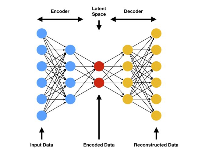
auoteencoder是深度学习的一类算法之一,由encoder, latent space和decoder组成(见下图)。更多知识分享请到 https://zouhua.top/。
packages
# Helper packages
library(dplyr)    # for data manipulation
library(ggplot2)  # for data visualization

# Modeling packages
library(h2o)  # for fitting autoencoders
train data
mnist <- dslabs::read_mnist()
names(mnist)
initialize H2O
h2o.no_progress()  # turn off progress bars
h2o.init(max_mem_size = "5g")  # initialize H2O instance
H2O is not running yet, starting it now...

Note:  In case of errors look at the following log files:
    C:\Users\zouhu\AppData\Local\Temp\Rtmp4APVUM\file521043104b5e/h2o_zouhua_started_from_r.out
    C:\Users\zouhu\AppData\Local\Temp\Rtmp4APVUM\file521021935c59/h2o_zouhua_started_from_r.err

java version "1.8.0_231"
Java(TM) SE Runtime Environment (build 1.8.0_231-b11)
Java HotSpot(TM) 64-Bit Server VM (build 25.231-b11, mixed mode)

Starting H2O JVM and connecting: . Connection successful!

R is connected to the H2O cluster:
    H2O cluster uptime:         5 seconds 583 milliseconds
    H2O cluster timezone:       Asia/Shanghai
    H2O data parsing timezone:  UTC
    H2O cluster version:        3.32.0.1
    H2O cluster version age:    2 months and 30 days
    H2O cluster name:           H2O_started_from_R_zouhua_vrf494
    H2O cluster total nodes:    1
    H2O cluster total memory:   4.44 GB
    H2O cluster total cores:    6
    H2O cluster allowed cores:  6
    H2O cluster healthy:        TRUE
    H2O Connection ip:          localhost
    H2O Connection port:        54321
    H2O Connection proxy:       NA
    H2O Internal Security:      FALSE
    H2O API Extensions:         Amazon S3, Algos, AutoML, Core V3, TargetEncoder, Core V4
    R Version:                  R version 4.0.2 (2020-06-22)
Comparing PCA to an autoencoder
# Convert mnist features to an h2o input data set
features <- as.h2o(mnist$train$images)

# Train an autoencoder
ae1 <- h2o.deeplearning(
  x = seq_along(features),
  training_frame = features,
  autoencoder = TRUE,
  hidden = 2,
  activation = 'Tanh',
  sparse = TRUE
)

# Extract the deep features
ae1_codings <- h2o.deepfeatures(ae1, features, layer = 1)
ae1_codings
Stacked autoencoders
# Hyperparameter search grid
hyper_grid <- list(hidden = list(
  c(50),
  c(100),
  c(300, 100, 300),
  c(100, 50, 100),
  c(250, 100, 50, 100, 250)
))

# Execute grid search
ae_grid <- h2o.grid(
  algorithm = 'deeplearning',
  x = seq_along(features),
  training_frame = features,
  grid_id = 'autoencoder_grid',
  autoencoder = TRUE,
  activation = 'Tanh',
  hyper_params = hyper_grid,
  sparse = TRUE,
  ignore_const_cols = FALSE,
  seed = 123
)

# Print grid details
h2o.getGrid('autoencoder_grid', sort_by = 'mse', decreasing = FALSE)
visualization
# Get sampled test images
index <- sample(1:nrow(mnist$test$images), 4)
sampled_digits <- mnist$test$images[index, ]
colnames(sampled_digits) <- paste0("V", seq_len(ncol(sampled_digits)))

# Predict reconstructed pixel values
best_model_id <- ae_grid@model_ids[[1]]
best_model <- h2o.getModel(best_model_id)
reconstructed_digits <- predict(best_model, as.h2o(sampled_digits))
names(reconstructed_digits) <- paste0("V", seq_len(ncol(reconstructed_digits)))

combine <- rbind(sampled_digits, as.matrix(reconstructed_digits))

# Plot original versus reconstructed
par(mfrow = c(1, 3), mar=c(1, 1, 1, 1))
layout(matrix(seq_len(nrow(combine)), 4, 2, byrow = FALSE))
for(i in seq_len(nrow(combine))) {
  image(matrix(combine[i, ], 28, 28)[, 28:1], xaxt="n", yaxt="n")
}
ANN2实现
Artificial Neural Networks package for R的优势
Easy to use interface - defining and training neural nets with a single function call!
Activation functions: tanh, sigmoid, relu, linear, ramp, step
Loss functions: log, squared, absolute, huber, pseudo-huber
Regularization: L1, L2
Optimizers: sgd, sgd w/ momentum, RMSprop, ADAM
Plotting functions for visualizing encodings, reconstructions and loss (training and validation)
Helper functions for predicting, reconstructing, encoding and decoding
Reading and writing the trained model from / to disk
Access to model parameters and low-level Rcpp module methods
- neuralnetwork() 神经网络
library(ANN2)

# Prepare test and train sets
random_idx <- sample(1:nrow(iris), size = 145)
X_train    <- iris[random_idx, 1:4]
y_train    <- iris[random_idx, 5]
X_test     <- iris[setdiff(1:nrow(iris), random_idx), 1:4]
y_test     <- iris[setdiff(1:nrow(iris), random_idx), 5]

# Train neural network on classification task
NN <- neuralnetwork(X = X_train,
                    y = y_train,
                    hidden.layers = c(5, 5),
                    optim.type = 'adam',
                    n.epochs = 5000)

# Predict the class for new data points
predict(NN, X_test)

# $predictions
# [1] "setosa"     "setosa"     "setosa"     "versicolor"     "versicolor"
#
# $probabilities
#      class_setosa class_versicolor class_virginica
# [1,] 0.9998184126     0.0001814204    1.670401e-07
# [2,] 0.9998311154     0.0001687264    1.582390e-07
# [3,] 0.9998280223     0.0001718171    1.605735e-07
# [4,] 0.0001074780     0.9997372337    1.552883e-04
# [5,] 0.0001077757     0.9996626441    2.295802e-04

# Plot the training and validation loss
plot(NN)

- autoencoder() 自编码
# Prepare test and train sets
random_idx <- sample(1:nrow(USArrests), size = 45)
X_train <- USArrests[random_idx,]
X_test <- USArrests[setdiff(1:nrow(USArrests), random_idx),]
# Define and train autoencoder
AE <- autoencoder(X = X_train,
hidden.layers = c(10,3,10),
loss.type = 'pseudo-huber',
optim.type = 'adam',
n.epochs = 5000)
# Reconstruct test data
reconstruct(AE, X_test)
# $reconstructed
# Murder Assault UrbanPop Rape
# [1,] 8.547431 243.85898 75.60763 37.791746
# [2,] 12.972505 268.68226 65.40411 29.475545
# [3,] 2.107441 78.55883 67.75074 15.040075
# [4,] 2.085750 56.76030 55.32376 9.346483
# [5,] 12.936357 252.09209 56.24075 24.964715
#
# $anomaly_scores
# [1] 398.926431 247.238111 11.613522 0.134633 1029.806121
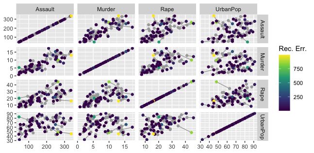
# Plot original points (grey) and reconstructions (colored) for training data
reconstruction_plot(AE, X_train)
Reference
Autoencoder
ANN2 tutorial
ANN2 github
参考文章如引起任何侵权问题,可以与我联系,谢谢。