逻辑回归
逻辑回归
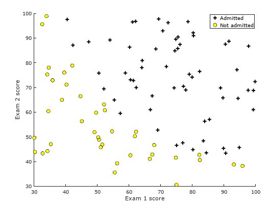
任务一 可视化数据(选择)
在ex2.m文件中已经导入了ex2data1.txt中的数据,其代码如下:
data = load('ex2data1.txt');
X = data(:, [1, 2]);
y = data(:, 3);
我们只需在plotData.m文件中,将plotData()函数代码补充完整,代码如下:
positive = find(y==1);
negative = find(y==0);

plot(X(positive, 1), X(positive, 2), 'k+', 'LineWidth', 2, 'MarkerSize', 7);
plot(X(negative, 1), X(negative, 2), 'ko', 'MarkerFaceColor', 'y','MarkerSize', 7);
其中,此代码中涉及到的plot()函数的应用可查看本人的Octave教程(四)或自行查阅相关文档。
运行该任务部分代码,其结果如下图所示:
任务二 代价函数与梯度下降算法
在ex2.m文件中已经将相关参数初始化代码以及函数调用代码写好,其代码如下:
[m, n] = size(X);

% Add intercept term to x and X_test
X = [ones(m, 1) X];

% Initialize fitting parameters
initial_theta = zeros(n + 1, 1);

% Compute and display initial cost and gradient
[cost, grad] = costFunction(initial_theta, X, y);
我们只需在costFunction.m将代价函数和梯度下降算法相关代码补充完整即可。不过在此之前,我们需要在sigmoid.m文件中将sigmoid()函数补充完整。
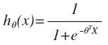
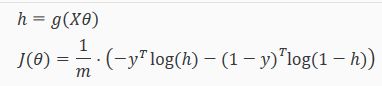
首先,我们将要用到的公式列举一下:
- 假设函数hθ(x):
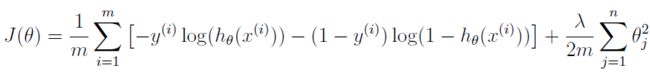
- 代价函数J(θ):

其向量化后为:
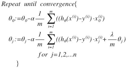
- 梯度下降算法:
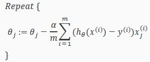
其向量化后为:
然后,我们在sigmoid.m文件中,根据假设函数hθ(x)公式键入如下代码:
g = 1 ./ (1+exp(-z));
最后,我们在costFunction.m文件中,将代价函数J(θ)和梯度下降算法分别补充完整,其代码分别如下:
代价函数J(θ)
J = (-y'*log(sigmoid(X*theta))-(1-y)'*log(1-sigmoid(X*theta))) / m;
梯度下降算法
grad = (X'*(sigmoid(X*theta)-y)) / m;
运行该部分代码,其结果为:
Cost at initial theta (zeros): 0.693147
Expected cost (approx): 0.693
Gradient at initial theta (zeros):
 -0.100000
 -12.009217
 -11.262842
Expected gradients (approx):
 -0.1000
 -12.0092
 -11.2628

Cost at test theta: 0.218330
Expected cost (approx): 0.218
Gradient at test theta:
 0.042903
 2.566234
 2.646797
Expected gradients (approx):
 0.043
 2.566
 2.647
任务三 高级优化算法
在ex2.m文件中已经将使用fminunc()函数的相关代码写好,我们只需运行即可,其代码如下:
%  Set options for fminunc
options = optimset('GradObj', 'on', 'MaxIter', 400);

%  Run fminunc to obtain the optimal theta
%  This function will return theta and the cost
[theta, cost] = ...
    fminunc(@(t)(costFunction(t, X, y)), initial_theta, options);

% Print theta to screen
fprintf('Cost at theta found by fminunc: %f\n', cost);
fprintf('Expected cost (approx): 0.203\n');
fprintf('theta: \n');
fprintf(' %f \n', theta);
fprintf('Expected theta (approx):\n');
fprintf(' -25.161\n 0.206\n 0.201\n');

% Plot Boundary
plotDecisionBoundary(theta, X, y);

% Put some labels
hold on;
% Labels and Legend
xlabel('Exam 1 score')
ylabel('Exam 2 score')

% Specified in plot order
legend('Admitted', 'Not admitted')
hold off;
该任务运行结果为:
Cost at theta found by fminunc: 0.203498
Expected cost (approx): 0.203
theta:
 -25.161272
 0.206233
 0.201470
Expected theta (approx):
 -25.161
 0.206
 0.201

任务四 逻辑回归的预测
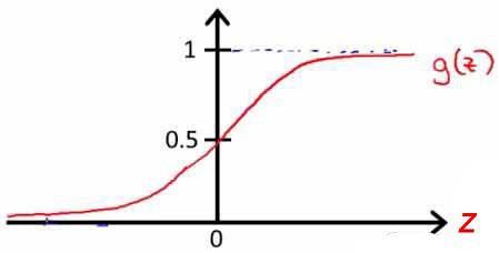
根据逻辑函数g(z)可知:
- 当z≥0.5时,我们可以预测y=1
- 当z﹤0.5时,我们可以预测y=0
因此,根据以上结论,我们可在predict.m文件中将predict()函数代码补充完整,其代码如下:
p(sigmoid( X * theta) >= 0.5) = 1;
p(sigmoid( X * theta) < 0.5) = 0;
此处代码可拆成如下代码便于理解:
k = find(sigmoid( X * theta) >= 0.5 );
p(k)= 1;

d = find(sigmoid( X * theta) < 0.5 );
p(d)= 0;
该任务的运行结果为:
For a student with scores 45 and 85, we predict an admission probability of 0.776289
Expected value: 0.775 +/- 0.002

Train Accuracy: 89.000000
Expected accuracy (approx): 89.0
正则化的逻辑回归
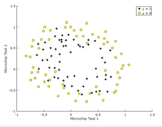
任务一 可视化数据
由于ex2_reg.m文件和plotData.m文件中都已将相关代码写好,我们只需运行该任务代码即可,其运行结果为:
任务二 代价函数与梯度下降算法
正则化的代价函数J(θ):
正则化的梯度下降算法:
根据上述公式,我们可在costFunctionReg.m文件中将代价函数和梯度下降算法补充完整,其代码如下:
theta_s = [0; theta(2:end)];
J= (-1 * sum( y .* log( sigmoid(X*theta) ) + (1 - y ) .* log( (1 - sigmoid(X*theta)) ) ) / m) + (lambda / (2*m) * (theta_s' * theta_s));
grad = ( X' * (sigmoid(X*theta) - y ) )/ m + ((lambda/m)*theta_s);
其运行结果为:
Cost at initial theta (zeros): 0.693147
Expected cost (approx): 0.693
Gradient at initial theta (zeros) - first five values only:
 0.008475
 0.018788
 0.000078
 0.050345
 0.011501
Expected gradients (approx) - first five values only:
 0.0085
 0.0188
 0.0001
 0.0503
 0.0115

Program paused. Press enter to continue.

Cost at test theta (with lambda = 10): 3.164509
Expected cost (approx): 3.16
Gradient at test theta - first five values only:
 0.346045
 0.161352
 0.194796
 0.226863
 0.092186
Expected gradients (approx) - first five values only:
 0.3460
 0.1614
 0.1948
 0.2269
 0.0922
任务三 高级优化算法
其代码已经写好,我们只需运行即可,其结果为:
Train Accuracy: 83.050847
Expected accuracy (with lambda = 1): 83.1 (approx)

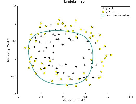
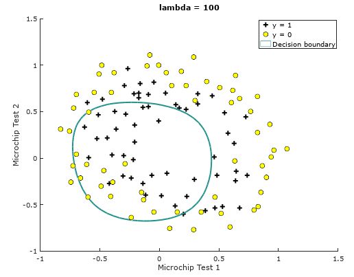
任务四 选择正则化参数λ(选做)
我们分别令正则化参数λ=0, 10, 100,其结果分别为:
λ=0
Train Accuracy: 86.440678

λ=10
Train Accuracy: 74.576271
λ=100
Train Accuracy: 61.016949
其中,关于图像绘制请自行查看plotDecisionBoundary.m文件。