Deep learning：三十七(Deep learning中的优化方法)

 

　　内容：

　　本文主要是参考论文：On optimization methods for deep learning，文章内容主要是笔记SGD（随机梯度下降），LBFGS（受限的BFGS），CG（共轭梯度法）三种常见优化算法的在deep learning体系中的性能。下面是一些读完的笔记。

　　SGD优点：实现简单，当训练样本足够多时优化速度非常快。

　　SGD缺点：需要人为调整很多参数，比如学习率，收敛准则等。另外，它是序列的方法，不利于GPU并行或分布式处理。

　　各种deep learning中常见方法（比如说Autoencoder，RBM，DBN，ICA，Sparse coding）的区别是：目标函数形式不同。这其实才是最本质的区别，由于目标函数的不同导致了对其优化的方法也可能会不同，比如说RBM中目标函数跟网络能量有关，采用CD优化的，而Autoencoder目标函数为理论输出和实际输出的MSE，由于此时的目标函数的偏导可以直接被计算，所以可以用LBFGS，CG等方法优化，其它的类似。所以不能单从网络的结构来判断其属于Deep learning中的哪种方法，比如说我单独给定64-100的2层网络，你就无法知道它属于deep learning中的哪一种方法，因为这个网络既可以用RBM也可以用Autoencoder来训练。

　　作者通过实验得出的结论是：不同的优化算法有不同的优缺点，适合不同的场合，比如LBFGS算法在参数的维度比较低（一般指小于10000维）时的效果要比SGD（随机梯度下降）和CG（共轭梯度下降）效果好，特别是带有convolution的模型。而针对高维的参数问题，CG的效果要比另2种好。也就是说一般情况下，SGD的效果要差一些，这种情况在使用GPU加速时情况一样，即在GPU上使用LBFGS和CG时，优化速度明显加快，而SGD算法优化速度提高很小。在单核处理器上，LBFGS的优势主要是利用参数之间的2阶近视特性来加速优化，而CG则得得益于参数之间的共轭信息，需要计算器Hessian矩阵。

　　不过当使用一个大的minibatch且采用线搜索的话，SGD的优化性能也会提高。

　　在单核上比较SGD，LBFGS，CG三种算法的优化性能，当针对Autoencoder模型。结果如下：

 　　

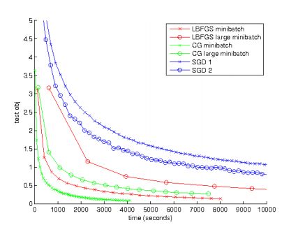
　　可以看出，SGD效果最差。

　　同样的情况下，训练的是Sparse autoencoder模型的比较情况如下：

 　　

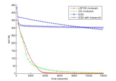
　　这时SGD的效果更差。这主要原因是LBFGS和CG能够使用大的minibatch数据来估算每个节点的期望激发值，这个值是可以用来约束该节点的稀疏特性的，而SGD需要去估计噪声信息。

　　当然了作者还有在GUP，convolution上也做了不少实验。

　　最后，作者训练了一个2隐含层（这2层不算pooling层）的Sparse autocoder网络，并应用于MNIST上，其识别率结果如下：

 　　

　　作者网站上给出了一些code，见deep autoencoder with L-BFGS。看着标题本以为code会实现deep convolution autoencoder pre-training和fine-tuning的，因为作者paper里面用的是convolution，阅读完code后发现其实现就是一个普通二层的autoencoder。看来还是得到前面博文第二个问题的答案：Deep learning：三十六(关于构建深度卷积SAE网络的一点困惑)。

 

　　下面是作者code主要部分的一些注释：

optimizeAutoencoderLBFGS.m(实现deep autoencoder网络的参数优化过程):

function [] = optimizeAutoencoderLBFGS(layersizes, datasetpath, ...

                                       finalObjective)

% train a deep autoencoder with variable hidden sizes

% layersizes : the sizes of the hidden layers. For istance, specifying layersizes =

%     [200 100] will create a network looks like input -> 200 -> 100 -> 200

%     -> output (same size as input). Notice the mirroring structure of the

%     autoencoders. Default layersizes = [2*3072 100]

% datasetpath: the path to the CIFAR dataset (where we find the *.mat

%     files). see loadData.m

% finalObjective: the final objective that you use to compare to

%                 terminate your optimization. To qualify, the objective

%                 function on the entire training set must be below this

%                 value.

%

% Author: Quoc V. Le ([email protected])

% 

%% Handle default parameters

if nargin < 3 || isempty(finalObjective)

    finalObjective = 70; % i am just making this up, the evaluation objective 

                         % will be much lower

end

if nargin < 2 || isempty(datasetpath)

  datasetpath = '.';

end

if nargin < 1 || isempty(layersizes)

  layersizes = [2*3072 100];

  layersizes = [200 100];

end



%% Load data

loadData %traindata 3072*10000的，每一列表示一个向量



%% Random initialization

initializeWeights;%看作者对应该部分的code，也没有感觉出convolution和pooling的影响啊，怎么它就连接起来了呢



%% Optimization: minibatch L-BFGS

% Q.V. Le, J. Ngiam, A. Coates, A. Lahiri, B. Prochnow, A.Y. Ng. 

% On optimization methods for deep learning. ICML, 2011



addpath minFunc/

options.Method = 'lbfgs'; 

options.maxIter = 20;      

options.display = 'on';

options.TolX = 1e-3;



perm = randperm(size(traindata,2));

traindata = traindata(:,perm);% 将训练样本随机排列

batchSize = 1000;%因为总共样本数为10000个，所以分成了10个批次

maxIter = 20;

for i=1:maxIter    

    startIndex = mod((i-1) * batchSize, size(traindata,2)) + 1;

    fprintf('startIndex = %d, endIndex = %d\n', startIndex, startIndex + batchSize-1);

    data = traindata(:, startIndex:startIndex + batchSize-1); 

    [theta, obj] = minFunc( @deepAutoencoder, theta, options, layersizes, ...

                            data);

    if obj <= finalObjective % use the minibatch obj as a heuristic for stopping

                             % because checking the entire dataset is very

                             % expensive

        % yes, we should check the objective for the entire training set        

        trainError = deepAutoencoder(theta, layersizes, traindata);

        if trainError <= finalObjective

            % now your submission is qualified

            break

        end

    end

end



%% write to text files so that we can test your program

writeToTextFiles;

 

deepAutoencoder.m:（深度网络代价函数及其导数的求解函数）:

function [cost,grad] = deepAutoencoder(theta, layersizes, data)

% cost and gradient of a deep autoencoder 

% layersizes is a vector of sizes of hidden layers, e.g., 

% layersizes[2] is the size of layer 2

% this does not count the visible layer

% data is the input data, each column is an example

% the activation function of the last layer is linear, the activation

% function of intermediate layers is the hyperbolic tangent function



% WARNING: the code is optimized for ease of implemtation and

% understanding, not speed nor space



%% FORCING THETA TO BE IN MATRIX FORMAT FOR EASE OF UNDERSTANDING

% Note that this is not optimized for space, one can just retrieve W and b

% on the fly during forward prop and backprop. But i do it here so that the

% readers can understand what's going on

layersizes = [size(data,1) layersizes];

l = length(layersizes);

lnew = 0;

for i=1:l-1

    lold = lnew + 1;

    lnew = lnew + layersizes(i) * layersizes(i+1);

    W{i} = reshape(theta(lold:lnew), layersizes(i+1), layersizes(i));

    lold = lnew + 1;

    lnew = lnew + layersizes(i+1);

    b{i} = theta(lold:lnew);

end

% handle tied-weight stuff

j = 1;

for i=l:2*(l-1)

    lold = lnew + 1;

    lnew = lnew + layersizes(l-j);

    W{i} = W{l - j}'; %直接用encoder中对应的转置即可

    b{i} = theta(lold:lnew);

    j = j + 1;

end

assert(lnew == length(theta), 'Error: dimensions of theta and layersizes do not match\n')





%% FORWARD PROP

for i=1:2*(l-1)-1

    if i==1

        [h{i} dh{i}] = tanhAct(bsxfun(@plus, W{i}*data, b{i}));

    else

        [h{i} dh{i}] = tanhAct(bsxfun(@plus, W{i}*h{i-1}, b{i}));

    end

end

h{i+1} = linearAct(bsxfun(@plus, W{i+1}*h{i}, b{i+1}));



%% COMPUTE COST

diff = h{i+1} - data; 

M = size(data,2); 

cost = 1/M * 0.5 * sum(diff(:).^2);% 纯粹标准的autoencoder，不加其它比如sparse限制



%% BACKPROP

if nargout > 1

    outderv = 1/M * diff;    

    for i=2*(l-1):-1:2

        Wgrad{i} = outderv * h{i-1}';

        bgrad{i} = sum(outderv,2);        

        outderv = (W{i}' * outderv) .* dh{i-1};        

    end

    Wgrad{1} = outderv * data';

    bgrad{1} = sum(outderv,2);

        

    % handle tied-weight stuff        

    j = 1;

    for i=l:2*(l-1)

        Wgrad{l-j} = Wgrad{l-j} + Wgrad{i}';

        j = j + 1;

    end

    % dump the results to the grad vector

    grad = zeros(size(theta));

    lnew = 0;

    for i=1:l-1

        lold = lnew + 1;

        lnew = lnew + layersizes(i) * layersizes(i+1);

        grad(lold:lnew) = Wgrad{i}(:);

        lold = lnew + 1;

        lnew = lnew + layersizes(i+1);

        grad(lold:lnew) = bgrad{i}(:);

    end

    j = 1;

    for i=l:2*(l-1)

        lold = lnew + 1;

        lnew = lnew + layersizes(l-j);

        grad(lold:lnew) = bgrad{i}(:);

        j = j + 1;

    end

end 

end



%% USEFUL ACTIVATION FUNCTIONS

function [a da] = sigmoidAct(x)



a = 1 ./ (1 + exp(-x));

if nargout > 1

    da = a .* (1-a);

end

end



function [a da] = tanhAct(x)

a = tanh(x);

if nargout > 1

    da = (1-a) .* (1+a);

end

end



function [a da] = linearAct(x)

a = x;

if nargout > 1

    da = ones(size(a));

end

end

 

initializeWeights.m（参数初始化赋值，虽然是随机，但是有一定要求）:

%% Random initialization

% X. Glorot, Y. Bengio. 

% Understanding the dif铿乧ulty of training deep feedforward neural networks.

% AISTATS 2010.

% QVL: this initialization method appears to perform better than 

% theta = randn(d,1);

s0 = size(traindata,1);% s0涓烘牱鏈殑缁存暟

layersizes = [s0 layersizes];%输入层-hidden1-hidden2，这里是3072-6144-100

l = length(layersizes);%缃戠粶涓殑灞傛暟锛屼笉鍖呭惈瑙ｇ爜閮ㄥ垎锛屽鏋滄槸2涓殣鍚眰鐨勮瘽锛岃繖閲宭=3

lnew = 0;

for i=1:l-1%1到3之间

    lold = lnew + 1;

    lnew = lnew + layersizes(i) * layersizes(i+1);

    r  = sqrt(6) / sqrt(layersizes(i+1)+layersizes(i));   

    A = rand(layersizes(i+1), layersizes(i))*2*r - r; %reshape(theta(lold:lnew), layersizes(i+1), layersizes(i));

    theta(lold:lnew) = A(:); %相当于权值W的赋值

    lold = lnew + 1;

    lnew = lnew + layersizes(i+1);

    A = zeros(layersizes(i+1),1);

    theta(lold:lnew) = A(:);%相当于偏置值b的赋值

end %以上是encoder部分

j = 1;

for i=l:2*(l-1) %1到4之间，下面开始decoder部分

    lold = lnew + 1;

    lnew = lnew + layersizes(l-j);

    theta(lold:lnew)= zeros(layersizes(l-j),1);

    j = j + 1;

end

theta = theta';

layersizes = layersizes(2:end); %去除输入层

 

 

　　参考资料：

　　Le, Q. V., et al. (2011). On optimization methods for deep learning. Proc. of ICML.

     deep autoencoder with L-BFGS

      Deep learning：三十六(关于构建深度卷积SAE网络的一点困惑)