【精品系列】【机器学习实战】【完整版】区域房价中位数预测(挑战全网最全,没有之一,另附完整代码)
参照《机器学习实战》第二版
1、下载数据
import os
import tarfile
import urllib.request

DOWNLOAD_ROOT = "https://raw.githubusercontent.com/ageron/handson-ml2/master/"
HOUSING_PATH = os.path.join("datasets", "housing")
HOUSING_URL = DOWNLOAD_ROOT + "datasets/housing/housing.tgz"

def fetch_housing_data(housing_url=HOUSING_URL, housing_path=HOUSING_PATH):
    if not os.path.isdir(housing_path):
        os.makedirs(housing_path)
    tgz_path = os.path.join(housing_path, "housing.tgz")
    urllib.request.urlretrieve(housing_url, tgz_path)
    housing_tgz = tarfile.open(tgz_path)
    housing_tgz.extractall(path=housing_path)
    housing_tgz.close()
fetch_housing_data()
2、读取下载的数据
import pandas as pd

def load_housing_data(housing_path=HOUSING_PATH):
    csv_path = os.path.join(housing_path, "housing.csv")
    return pd.read_csv(csv_path)
2.1、数据显示
housing = load_housing_data()
housing.head()  # 默认显示前五列
| longitude | latitude | housing_median_age | total_rooms | total_bedrooms | population | households | median_income | median_house_value | ocean_proximity | |
|---|---|---|---|---|---|---|---|---|---|---|
| 0 | -122.23 | 37.88 | 41.0 | 880.0 | 129.0 | 322.0 | 126.0 | 8.3252 | 452600.0 | NEAR BAY |
| 1 | -122.22 | 37.86 | 21.0 | 7099.0 | 1106.0 | 2401.0 | 1138.0 | 8.3014 | 358500.0 | NEAR BAY |
| 2 | -122.24 | 37.85 | 52.0 | 1467.0 | 190.0 | 496.0 | 177.0 | 7.2574 | 352100.0 | NEAR BAY |
| 3 | -122.25 | 37.85 | 52.0 | 1274.0 | 235.0 | 558.0 | 219.0 | 5.6431 | 341300.0 | NEAR BAY |
| 4 | -122.25 | 37.85 | 52.0 | 1627.0 | 280.0 | 565.0 | 259.0 | 3.8462 | 342200.0 | NEAR BAY |
2.2、查看每列属性
housing.info()
RangeIndex: 20640 entries, 0 to 20639
Data columns (total 10 columns):
 #   Column              Non-Null Count  Dtype
---  ------              --------------  -----
 0   longitude           20640 non-null  float64
 1   latitude            20640 non-null  float64
 2   housing_median_age  20640 non-null  float64
 3   total_rooms         20640 non-null  float64
 4   total_bedrooms      20433 non-null  float64
 5   population          20640 non-null  float64
 6   households          20640 non-null  float64
 7   median_income       20640 non-null  float64
 8   median_house_value  20640 non-null  float64
 9   ocean_proximity     20640 non-null  object
dtypes: float64(9), object(1)
memory usage: 1.6+ MB
2.3、查看某列数值统计
housing["ocean_proximity"].value_counts()
<1H OCEAN     9136
INLAND        6551
NEAR OCEAN    2658
NEAR BAY      2290
ISLAND           5
Name: ocean_proximity, dtype: int64
2.4、查看数值列属性摘要
housing.describe()
| longitude | latitude | housing_median_age | total_rooms | total_bedrooms | population | households | median_income | median_house_value | |
|---|---|---|---|---|---|---|---|---|---|
| count | 20640.000000 | 20640.000000 | 20640.000000 | 20640.000000 | 20433.000000 | 20640.000000 | 20640.000000 | 20640.000000 | 20640.000000 |
| mean | -119.569704 | 35.631861 | 28.639486 | 2635.763081 | 537.870553 | 1425.476744 | 499.539680 | 3.870671 | 206855.816909 |
| std | 2.003532 | 2.135952 | 12.585558 | 2181.615252 | 421.385070 | 1132.462122 | 382.329753 | 1.899822 | 115395.615874 |
| min | -124.350000 | 32.540000 | 1.000000 | 2.000000 | 1.000000 | 3.000000 | 1.000000 | 0.499900 | 14999.000000 |
| 25% | -121.800000 | 33.930000 | 18.000000 | 1447.750000 | 296.000000 | 787.000000 | 280.000000 | 2.563400 | 119600.000000 |
| 50% | -118.490000 | 34.260000 | 29.000000 | 2127.000000 | 435.000000 | 1166.000000 | 409.000000 | 3.534800 | 179700.000000 |
| 75% | -118.010000 | 37.710000 | 37.000000 | 3148.000000 | 647.000000 | 1725.000000 | 605.000000 | 4.743250 | 264725.000000 |
| max | -114.310000 | 41.950000 | 52.000000 | 39320.000000 | 6445.000000 | 35682.000000 | 6082.000000 | 15.000100 | 500001.000000 |
- 上面看到
total_bedrooms这一列的count的数值为20433而不是20640,是因为不统计为空的单元格,所以后面需要处理为空的数据。 std行:显示的是标准差,用来测量数值的离散程度,也就是方差的平方根,一般符合高斯分布- 25%、50%、75%:显示相应的百分位数,表示一组观测值中给定百分比的观测值都低于该值;50% 即 中位数。
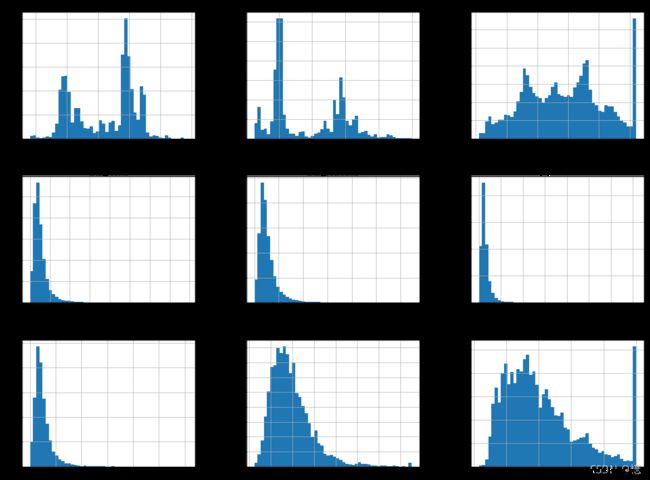
2.5、快速了解数组类型的方法(直方图)
%matplotlib inline
import matplotlib.pyplot as plt
housing.hist(bins=50, figsize=(20, 15))
plt.show()
3、创建测试集
理论上,创建测试集非常简单,只需要随机选择一些实例,通常是数据集的20%(如果数据量巨大,比例将更小)
- 为了即使在更新数据集之后也有一个稳定的训练测试分割,常见的解决方案是每个实例都使用一个
标识符来决定是否进入测试集(假定每个实例都一个唯一且不变的标识符) - 你可以计算每个实例的标识符的哈希值,如果这个哈希值小于或等于最大哈希值的20%,则将该实例放入测试集。这样可以保证测试集在多个运行里都是一致的,即便更新数据集也依然一致。新实例的20%将被放如新的测试集,而之前训练集中的实例也不会被放入新测试集。
3.1、手动随机生成
from zlib import crc32
import numpy as np


def test_set_check(identifier, test_ratio):
    return crc32(np.int64(identifier)) & 0xffffffff < test_ratio * 2**32


def splet_train_test_by_id(data, test_ratio, id_column):
    ids = data[id_column]
    in_test_set = ids.apply(lambda id_: test_set_check(id_, test_ratio))
    return data.loc[~in_test_set], data.loc[in_test_set]
- housing 数据集没有标识符列。最简单的解决方法是使用索引作为 ID
housing_with_id = housing.reset_index()
train_set, test_set = splet_train_test_by_id(housing_with_id, 0.2, "index")
3.2、使用 Scikit-Learn 提供的方法 train_test_split 随机生成
- 最简单的方法就是使用:train_test_split(),它与前面定义的 split_train_test() 几乎相同,除了几个额外特征。
from sklearn.model_selection import train_test_split

# random_state: 设置随机生成器种子
train_set, test_set = train_test_split(housing, test_size=0.2, random_state=42)
- 到目前为止,我们考虑的是纯随机的抽样方法。如果数据集足够庞大(特别是相较于属性的数量而言),这种方法通常不错
- 如果不是,则有可能会导致明显的抽样偏差。即 应该按照比例分层抽样。
如果你咨询专家,他们会告诉你,要预测房价中位数,收入中位数是个非常重要的属性。于是你希望确保在收入属性上,测试集能够代表整个数据集中各种不同类型的收入。
我们由上面直方图可以看到:大部分收入中位数值聚集在1.5~6左右,但也有一部分超过了6,在数据集中,每个层都要有足够数量的数据,这一点至关重要,不然数据不足的层,其重要程度佷有可能会被错估。
3.3、使用 Scikit-Learn 提供的方法 StratifiedShuffleSplit 按类别比例生成
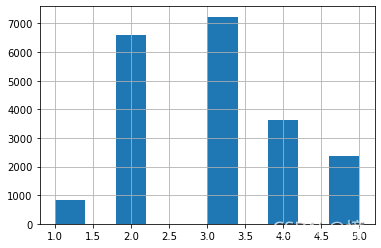
# 用 pd.cut() 来创建 5个收入类别属性(用 1~5 来做标签),0~1.5是类别 1, 1.5~3是类别2
# np.inf 代表无穷大
housing["income_cat"] = pd.cut(housing["median_income"],
                               bins=[0, 1.5, 3, 4.5, 6, np.inf],
                               labels=[1, 2, 3, 4, 5])
housing["income_cat"].hist()
现在根据收入类进行分层抽样,使用 Scikit-Learn 的 StratifiedShuffleSplit
from sklearn.model_selection import StratifiedShuffleSplit

split = StratifiedShuffleSplit(n_splits=1, test_size=0.2, random_state=42)
for train_index, test_index in split.split(housing, housing["income_cat"]):
    strat_train_set = housing.loc[train_index]
    strat_test_set = housing.loc[test_index]
看看上面运行是否如我们所料
compare_pd = pd.DataFrame()
# 全部数据:按收入分类的比例
compare_pd["全部数据"] = housing["income_cat"].value_counts() / len(housing)
# 按收入分类的比例 获取测试集比例
compare_pd["分类抽样"] = strat_test_set["income_cat"].value_counts() / len(strat_test_set)
# 随机获取测试集比例
_, test_set = train_test_split(housing, test_size=0.2, random_state=42)
compare_pd["随机抽样"] = test_set["income_cat"].value_counts() / len(test_set)
compare_pd
| 全部数据 | 分类抽样 | 随机抽样 | |
|---|---|---|---|
| 3 | 0.350581 | 0.350533 | 0.358527 |
| 2 | 0.318847 | 0.318798 | 0.324370 |
| 4 | 0.176308 | 0.176357 | 0.167393 |
| 5 | 0.114438 | 0.114583 | 0.109496 |
| 1 | 0.039826 | 0.039729 | 0.040213 |
由上面数据我们看到,随机抽样的测试集,收入类别比例分布有些偏差。
现在可以删除 income_cat 属性,将数据恢复原样了:
for set_ in (strat_train_set, strat_test_set):
    set_.drop("income_cat", axis=1, inplace=True)
我们花了相当长的时间在测试集的生成上,理由很充分:这是及机器学习项目中经常忽视但是却至关重要的一部分。并且,当讨论到交叉验证时,这里谈到的许多想法也对其大有裨益。
4、从数据探索和可视化中获取洞见
如果训练集非常庞大,你可以抽样一个探索集,这样后面的操作更简单快捷一些,不过我们这个案例的数据集非常小,完全可以直接在整个训练集上操作。让我们先创建一个副本,这样可以随便尝试而不损害训练集:
housing = strat_train_set.copy()
4.1、将地理数据可视化
housing.plot(kind="scatter", x="longitude", y="latitude")

# alpha=0.1 可以更清楚的看出高密度数据点的位置
housing.plot(kind="scatter", x="longitude", y="latitude", alpha=0.1)

housing.plot(kind="scatter", x="longitude", y="latitude", alpha=0.4,
             s=housing["population"]/100, label="population", figsize=(10, 7),
             c="median_house_value", cmap=plt.get_cmap("jet"), colorbar=True)
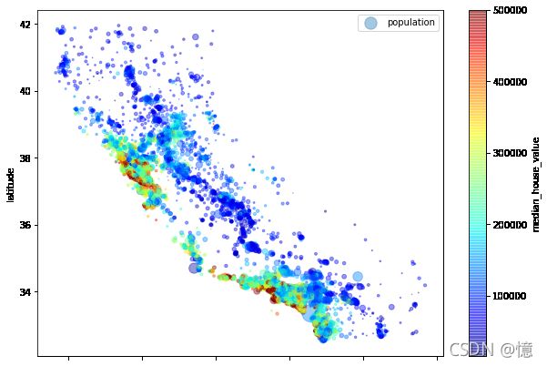
现在,再看看房价。每个圆的半径大小代表了每个区域的人口数量(选项 s),颜色代表价格(选项 c)。我们使用一个名叫jet的预定义颜色表(选项 cmap)来进行可视化,颜色范围从蓝(低)到红(高)
4.2、寻找相关性
由于数据集不太大,你可以使用 corr() 方法轻松计算出没对属性之间的标准相关系数(也称皮尔逊 r)
corr_matrix = housing.corr()
现在查看每个属性与房价中位数的相关性分别是多少:
corr_matrix["median_house_value"].sort_values(ascending=False)
median_house_value    1.000000
median_income         0.687160
total_rooms           0.135097
housing_median_age    0.114110
households            0.064506
total_bedrooms        0.047689
population           -0.026920
longitude            -0.047432
latitude             -0.142724
Name: median_house_value, dtype: float64
相关系数的范围从 -1 变化到 1。
-
越接近
1,表示有越强的正相关。当收入中位数上升时,房价中位数也趋于上升 -
越接近
-1,表示有越强的负相关。可以发现纬度和房价中位数呈现轻微的负相关,也就是说,越往北走,房价倾向于下降 -
越接近
0,表示两者之间没有线性相关性。可以发现纬度和房价中位数呈现轻微的负相关,也就是说,越往北走,房价倾向于下降
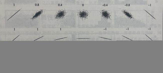
上图可知,相关系数仅测量线性相关性,所以她有可能彻底遗漏非线性相关性。注意最下面一排图像,他们的相关系数都是0,但是显然我们可以看出横轴和纵轴之间的关系并不是完全独立的。此外前两行,需要注意的是这个相关性跟斜率完全无关
还有一种方法可以检测属性之间的相关性,也就是使用pandas的scatter_matix函数,它会绘制出每个数值属性相对于其他数值属性的相关性。现在我们有11个数值属性,可以得到 11^2 = 121 个图像,这里我们只关注这些与房价中位数属性最相关的,可算作最有潜力的属性
from pandas.plotting import scatter_matrix

# 选择了相关性靠前的 4 个属性
attributes = ["median_house_value", "median_income", "total_rooms", "housing_median_age"]
scatter_matrix(housing[attributes], figsize=(12, 8))
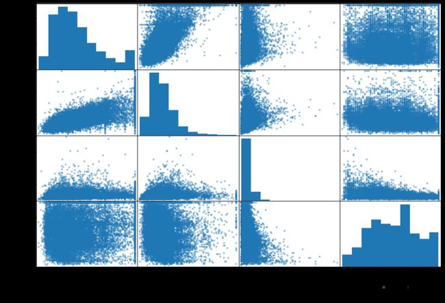
最有潜力能预测房价中位数的属性是收入中位数,所以我们放大开看看其相关属性的散点图
housing.plot(kind="scatter", x="median_income", y="median_house_value", alpha=0.1)
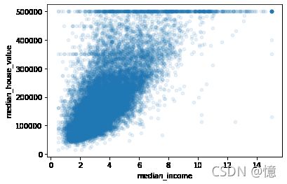
- 上图可以明显的看到上升趋势,并且点也不是太分散。
- 明显可以看到几条水平线,比如:50万、45万、35万、30万以下还有几条不太明显的线。
- 为了避免你的算法学习之后重现这些怪异数据,可以尝试删除这些相应区域。
4.3、试验不同属性的组合(为 5.3 自定义转换器的编写做准备)
应于发现其他有意思的数据关系。
# 房屋总数 / 住户
housing["rooms_per_household"] = housing["total_rooms"]/housing["households"]
# 卧室总数 / 房屋总数
housing["bedrooms_per_room"] = housing["total_bedrooms"]/housing["total_rooms"]
# 人口 / 住户
housing["population_per_household"]=housing["population"]/housing["households"]
corr_matrix = housing.corr()
corr_matrix["median_house_value"].sort_values(ascending=False)
median_house_value          1.000000
median_income               0.687160
rooms_per_household         0.146285
total_rooms                 0.135097
housing_median_age          0.114110
households                  0.064506
total_bedrooms              0.047689
population_per_household   -0.021985
population                 -0.026920
longitude                  -0.047432
latitude                   -0.142724
bedrooms_per_room          -0.259984
Name: median_house_value, dtype: float64
这一轮的探索不一定要多么彻底,关键是迈开这一步,快速获得洞见,这将有助于你获得非常非常好的第一个原型。这也是一个不断迭代的过程:
一旦你的原型产生并且开始运行,你可以分析它的输出以获得更多洞见,然后再次回到这个探索步骤。
5、机器学习算法的数据准备
现在,终于是时候给你的机器学习算法准备数据了。这里你应该编写函数来执行,而不是手动操作,原因如下:
- 你可以在任何数据集上轻松重现这些转换(比如,获得更新之后的数据集之后)
- 你可以逐渐建立起一个转换函数函数库,可以在以后的项目中重用。
- 你可以在实现系统中使用这些函数来转换新数据,在输入给算法。
- 你可以轻松尝试多种转换方式,查看哪种转换的组合效果最佳。
现在,让我们先回到一个干净的训练集(再次复制 strat_train_set),然后将预测期和标签分开,因为这里我们不一定对它们使用相同的转换方式(需要注意drop()会创建一个数据副本,但是不影响 strat_train_set):
housing = strat_train_set.drop("median_house_value", axis=1)
housing_labels = strat_train_set["median_house_value"].copy()
5.1、数据清理
5.1.1、常规方法(四种)
大部分的机器学习算法无法在缺失的特征上工作,所以我们要创建一些函数来辅助它。前面我们已经注意到total_bedrooms属性有部分值缺失,所以我们要先解决它。有一下三种选择:
- 放弃这些相应的区域
- 放弃整个属性
- 将缺失值设置为某个值(0、平均值或者中位数等)
- 将缺失值按分组设置为组内某个值(0、平均值或者中位数等)(我自己加的)
通过DataFrame的dropan()、drop()、fillan()、groupby()方法,可以轻松完成这些操作:
# 获取有缺失值的行,方便显示
sample_incomplete_rows = housing[housing.isnull().any(axis=1)].head()
sample_incomplete_rows
| longitude | latitude | housing_median_age | total_rooms | total_bedrooms | population | households | median_income | ocean_proximity | |
|---|---|---|---|---|---|---|---|---|---|
| 4629 | -118.30 | 34.07 | 18.0 | 3759.0 | NaN | 3296.0 | 1462.0 | 2.2708 | <1H OCEAN |
| 6068 | -117.86 | 34.01 | 16.0 | 4632.0 | NaN | 3038.0 | 727.0 | 5.1762 | <1H OCEAN |
| 17923 | -121.97 | 37.35 | 30.0 | 1955.0 | NaN | 999.0 | 386.0 | 4.6328 | <1H OCEAN |
| 13656 | -117.30 | 34.05 | 6.0 | 2155.0 | NaN | 1039.0 | 391.0 | 1.6675 | INLAND |
| 19252 | -122.79 | 38.48 | 7.0 | 6837.0 | NaN | 3468.0 | 1405.0 | 3.1662 | <1H OCEAN |
5.1.1.1、方法一:dropna()
sample_incomplete_rows.dropna(subset=["total_bedrooms"])
| longitude | latitude | housing_median_age | total_rooms | total_bedrooms | population | households | median_income | ocean_proximity |
|---|
5.1.1.2、方法二:drop()
sample_incomplete_rows.drop("total_bedrooms", axis=1)
| longitude | latitude | housing_median_age | total_rooms | population | households | median_income | ocean_proximity | |
|---|---|---|---|---|---|---|---|---|
| 4629 | -118.30 | 34.07 | 18.0 | 3759.0 | 3296.0 | 1462.0 | 2.2708 | <1H OCEAN |
| 6068 | -117.86 | 34.01 | 16.0 | 4632.0 | 3038.0 | 727.0 | 5.1762 | <1H OCEAN |
| 17923 | -121.97 | 37.35 | 30.0 | 1955.0 | 999.0 | 386.0 | 4.6328 | <1H OCEAN |
| 13656 | -117.30 | 34.05 | 6.0 | 2155.0 | 1039.0 | 391.0 | 1.6675 | INLAND |
| 19252 | -122.79 | 38.48 | 7.0 | 6837.0 | 3468.0 | 1405.0 | 3.1662 | <1H OCEAN |
5.1.1.3、方法三:fillna()
median = housing["total_bedrooms"].median()
sample_incomplete_rows["total_bedrooms"].fillna(median, inplace=True)
sample_incomplete_rows
| longitude | latitude | housing_median_age | total_rooms | total_bedrooms | population | households | median_income | ocean_proximity | |
|---|---|---|---|---|---|---|---|---|---|
| 4629 | -118.30 | 34.07 | 18.0 | 3759.0 | 433.0 | 3296.0 | 1462.0 | 2.2708 | <1H OCEAN |
| 6068 | -117.86 | 34.01 | 16.0 | 4632.0 | 433.0 | 3038.0 | 727.0 | 5.1762 | <1H OCEAN |
| 17923 | -121.97 | 37.35 | 30.0 | 1955.0 | 433.0 | 999.0 | 386.0 | 4.6328 | <1H OCEAN |
| 13656 | -117.30 | 34.05 | 6.0 | 2155.0 | 433.0 | 1039.0 | 391.0 | 1.6675 | INLAND |
| 19252 | -122.79 | 38.48 | 7.0 | 6837.0 | 433.0 | 3468.0 | 1405.0 | 3.1662 | <1H OCEAN |
5.1.1.4、方法四:groupby()
housing_group = housing.copy()
housing_group["income_cat"] = pd.cut(housing["median_income"],
                                     bins=[0, 1.5, 3, 4.5, 6, np.inf],
                                     labels=[1, 2, 3, 4, 5])
housing_group[housing.isnull().any(axis=1)].head()
| longitude | latitude | housing_median_age | total_rooms | total_bedrooms | population | households | median_income | ocean_proximity | income_cat | |
|---|---|---|---|---|---|---|---|---|---|---|
| 4629 | -118.30 | 34.07 | 18.0 | 3759.0 | NaN | 3296.0 | 1462.0 | 2.2708 | <1H OCEAN | 2 |
| 6068 | -117.86 | 34.01 | 16.0 | 4632.0 | NaN | 3038.0 | 727.0 | 5.1762 | <1H OCEAN | 4 |
| 17923 | -121.97 | 37.35 | 30.0 | 1955.0 | NaN | 999.0 | 386.0 | 4.6328 | <1H OCEAN | 4 |
| 13656 | -117.30 | 34.05 | 6.0 | 2155.0 | NaN | 1039.0 | 391.0 | 1.6675 | INLAND | 2 |
| 19252 | -122.79 | 38.48 | 7.0 | 6837.0 | NaN | 3468.0 | 1405.0 | 3.1662 | <1H OCEAN | 3 |
housing_group_median = housing_group.groupby("income_cat").transform(lambda x: x.fillna(x.median()))
housing_group_median[housing.isnull().any(axis=1)].head()
| longitude | latitude | housing_median_age | total_rooms | total_bedrooms | population | households | median_income | |
|---|---|---|---|---|---|---|---|---|
| 4629 | -118.30 | 34.07 | 18.0 | 3759.0 | 444.0 | 3296.0 | 1462.0 | 2.2708 |
| 6068 | -117.86 | 34.01 | 16.0 | 4632.0 | 427.0 | 3038.0 | 727.0 | 5.1762 |
| 17923 | -121.97 | 37.35 | 30.0 | 1955.0 | 427.0 | 999.0 | 386.0 | 4.6328 |
| 13656 | -117.30 | 34.05 | 6.0 | 2155.0 | 444.0 | 1039.0 | 391.0 | 1.6675 |
| 19252 | -122.79 | 38.48 | 7.0 | 6837.0 | 453.0 | 3468.0 | 1405.0 | 3.1662 |
如果选择方法三,你需要计算出训练集的中位数,然后用它填充训练集中的缺失值,但也别忘了保存这个计算出的中位数,因为后面可能需要用到。当重新评估系统时,你需要更换测试集中的缺失值;或者在系统上线时,需要使用新数据替代缺失值。
5.1.2、Scikit-Learn 提供的 SimpleImputer 方法
Scikit-Learn提供了一个非常容易上手的类来处理缺失值:SimpleImputer。使用方法如下:首先,你需要创建一个 SimpleImputer 实例,指定你要用属性的中位数值替换该属性的缺失值:
from sklearn.impute import SimpleImputer

imputer = SimpleImputer(strategy="median")
由于中位数只能在数值属性上计算,所以我们需要创建一个没有文本属性 ocean_proximity 的数据副本:
housing_num = housing.drop("ocean_proximity", axis=1)
使用fit()方法将imputer实例适配到训练数据:
imputer.fit(housing_num)
SimpleImputer(strategy='median')
这里imputer仅仅只是计算了每个属性的中位数值,并将结果储存在其实例变量statistics_中。虽然只是total_bedrooms这个属性存在缺失值,所以稳妥起见,还是将imputer应用于所有的数值属性:
# imputer 计算的每列中位数
imputer.statistics_
array([-118.51 , 34.26 , 29. , 2119.5 , 433. , 1164. , 408. , 3.5409])
# 直接计算的中位数
housing_num.median().values
array([-118.51 , 34.26 , 29. , 2119.5 , 433. , 1164. , 408. , 3.5409])
现在,你可以使用这个“训练有素”的imputer将缺失值替换成中位数从而完成训练集转换:
X = imputer.transform(housing_num)
type(X)
numpy.ndarray
结果是一个包含转换后特征的Numpy数组。如果你想将它放回Pandas DataFrame,也很简单:
housing_tr = pd.DataFrame(X, columns=housing_num.columns, index=housing_num.index)
housing_tr.loc[sample_incomplete_rows.index.values]
| longitude | latitude | housing_median_age | total_rooms | total_bedrooms | population | households | median_income | |
|---|---|---|---|---|---|---|---|---|
| 4629 | -118.30 | 34.07 | 18.0 | 3759.0 | 433.0 | 3296.0 | 1462.0 | 2.2708 |
| 6068 | -117.86 | 34.01 | 16.0 | 4632.0 | 433.0 | 3038.0 | 727.0 | 5.1762 |
| 17923 | -121.97 | 37.35 | 30.0 | 1955.0 | 433.0 | 999.0 | 386.0 | 4.6328 |
| 13656 | -117.30 | 34.05 | 6.0 | 2155.0 | 433.0 | 1039.0 | 391.0 | 1.6675 |
| 19252 | -122.79 | 38.48 | 7.0 | 6837.0 | 433.0 | 3468.0 | 1405.0 | 3.1662 |
5.2、处理文本和分类属性
5.2.1、使用 Scikit-Learn 的 OrdinalEncoder 类
到目前为止,我们只处理数值属性,但现在让我们看一下文本属性。在此数据集中,只有一个:ocean_proximity属性。前面我们一直到它不是任意文本,而是有限个可能的取值,每个值代表一类别。因此,此属性是分类属性。大多数机器学习算法更喜欢使用数字,因此让我们将这些类别从文件转到数字。为此,我们可以使用Scikit-Learn的OrdinalEncoder类:
housing["ocean_proximity"].value_counts()
<1H OCEAN     7276
INLAND        5263
NEAR OCEAN    2124
NEAR BAY      1847
ISLAND           2
Name: ocean_proximity, dtype: int64
from sklearn.preprocessing import OrdinalEncoder

housing_cat = housing[["ocean_proximity"]]
ordinal_encoder = OrdinalEncoder()
housing_cat_encoded = ordinal_encoder.fit_transform(housing_cat)
housing_cat_encoded[:10]
array([[0.],
       [0.],
       [4.],
       [1.],
       [0.],
       [1.],
       [0.],
       [1.],
       [0.],
       [0.]])
你可以使用categories_实例变量获取类别列表。这个列表包含每个类别属性的维一数组(在这种情况下,这个列表包含一个数组,因为只有一个类别属性):
ordinal_encoder.categories_
[array(['<1H OCEAN', 'INLAND', 'ISLAND', 'NEAR BAY', 'NEAR OCEAN'], dtype=object)]
这种表征方式产生的一个问题是,机器学习算法会认为两个相近的比值比两个离得较远的值更为相似一些,在某种情况下这是对的(比如一些有序类别,像“优”、“良”、“中”、“差”),但是对ocean_proximity而言情况并非如此(例如,类别0和类别4之间就比类别0和类别1之间的相似度更高)
5.2.2、使用 Scikit-Learn 的 OneHotEncoder 类
为了解决这个问题,常见的解决方案是给每个类别创建一个二进制的属性:
- 当类别是 “<1H OCEAN” 时,一个属性为 1(其他属性为 0)
- 当类别是 “INLAND” 时,另一个属性为 1(其他属性为 0)
- 以此类推
这就是独热编码,因为只有一个属性为 1(热),其他均为 0(冷)。新的属性有事成为哑(dummy)属性。Scikit-Learn的OneHotEncoder编码器,可以将整数类别转换为独热向量(新版本支持其他类别转换)。我们用它来将类别编码为独热向量。
from sklearn.preprocessing import OneHotEncoder

cat_encoder = OneHotEncoder()
housing_cat_1hot = cat_encoder.fit_transform(housing_cat)
housing_cat_1hot
<16512x5 sparse matrix of type ''
	with 16512 stored elements in Compressed Sparse Row format>
<16512x5 ‘
’ 类型的稀疏矩阵以压缩稀疏行格式存储 16512 个元素>
注意到这里的输出是一个SciPy稀疏矩阵,而不是一个NumPy数组。当你有成千上万个类别属性时,这个函数会非常有用。因为在独热编码完成之后,我们会得到一个几千列的矩阵,并且全部是0,每行仅有一个1。占用大量内存来储存0是一件非常浪费的事情,因此稀疏矩阵选择仅储存非零元素的位置。而你依旧可以像使用一个普通的二维数组那样来使用它。
如果你想把它转成一个(密集的)NumPy 数组,只需要调用toarray()方法即可:
housing_cat_1hot.toarray()
array([[1., 0., 0., 0., 0.],
       [1., 0., 0., 0., 0.],
       [0., 0., 0., 0., 1.],
       ...,
       [0., 1., 0., 0., 0.],
       [1., 0., 0., 0., 0.],
       [0., 0., 0., 1., 0.]])
再次使用编码器的categories_实例变量获取类别列表:
cat_encoder.categories_
[array(['<1H OCEAN', 'INLAND', 'ISLAND', 'NEAR BAY', 'NEAR OCEAN'], dtype=object)]
5.3、自定义转换器
虽然Scikit-Learn提供了许多有用的转换器,但是你依然需要为一些诸如自定义清理操作或组合特定属性等任务编写自己的转换器。你当然希望让自己的转换器与Scikit-Learn自身功能(比如流水线)无缝衔接,而由于Scikit-Learn依赖于鸭子类型的编译,而不是继承,所以你所需要的只是创建一个类,然后应用一下三种方法:fit()(返回self)、transform()、fit_transform()。
你可以通过添加TransformerMixin作为基类,直接得到最后一种方法。同时,如果添加BaseEstimator作为基类(并在构造函数中避免 *args和**kargs),你还能额外获得两个非常有用的自动调整超参数的方法(get_params()和set_params())。
例如,我们前面讨论过得组合属性,这里有个简单的转换器类,用来添加组合后的属性:
from sklearn.base import BaseEstimator, TransformerMixin
# 对应数据所在列的位置,从0开始计数
# rooms_ix, bedroom_ix, population_ix, households_ix = 3, 4, 5, 6
col_names = "total_rooms", "total_bedrooms", "population", "households"
# get the column indices
rooms_ix, bedrooms_ix, population_ix, households_ix = [housing.columns.get_loc(c) for c in col_names]
class CombinedAttributesAdder(BaseEstimator, TransformerMixin):
def __init__(self, add_bedroom_per_room=True):
# 没有 *args 和 **kargs
self.add_bedroom_per_room = add_bedroom_per_room
def fit(self, X, y=None):
# 不做任何处理
return self
def transform(self, X):
"""
X[:, rooms_ix]:X数组,":"所有行,取rooms_ix列的数据(即,取第rooms_ix列的全部数据,从0开始计数)
------------
np.r_是按列连接两个矩阵,就是把两矩阵上下相加,要求列数相等。
np.c_是按行连接两个矩阵,就是把两矩阵左右相加,要求行数相等。即添加计算后的新列数据
例:
a = np.array([[1, 2, 3],
[7,8,9]])
b = np.array([[4,5,6],
[1,2,3]])
c = np.c_[a,b]
>>> print(c)
array([[1, 2, 3, 4, 5, 6],
[7, 8, 9, 1, 2, 3]])
"""
rooms_per_household = X[:, rooms_ix] / X[:, households_ix] # 即 第 3 列数据 ÷ 第 6 列数据
population_per_household = X[:, population_ix] / X[:, households_ix]
if self.add_bedroom_per_room:
bedrooms_per_room = X[:, bedroom_ix] / X[:, rooms_ix]
return np.c_[X, rooms_per_household, population_per_household, bedrooms_per_room]
else:
return np.c_[X, rooms_per_household, population_per_household]
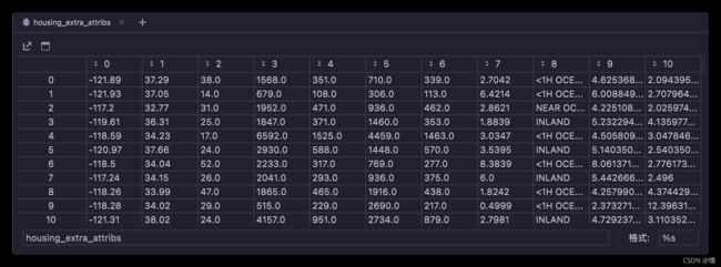
attr_adder = CombinedAttributesAdder(add_bedroom_per_room=False)
housing_extra_attribs = attr_adder.transform(housing.values)
- housing
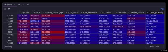
- housing.values(即 X)
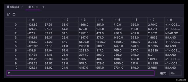
- housing_extra_attribs(即 转换结果)
本案例中,转换器有一个超参数add_bedroom_per_room默认设置为True(提供合理的默认值通用是很有帮助的)。
- 这个参数可以让你轻松知晓添加这个属性是否有助于机器学习算法。
- 更一般地,如果你对数据准备的步骤没有充分的信心,就可以添加这个超参数来进行把关。
- 这些数据准备步骤的执行越是自动化,你自动尝试的组合也就越多,从而有更大可能从中找到一个重要的组合(还节省了大量时间)。
5.4、特征缩放
最重要也最需要应用到数据上的转换就是特征缩放。如果输入的数值属性具有非常大的比例差异,往往会导致机器学习算法的性能表现不佳,当然也有极少数特例。案例中的房屋数据就是这样:房屋总数的范围从 6~39320,而收入中位数的范围是 0~15。注意,目标值通常不需要缩放。
同比例缩放所有属性的两种常用方法是最小值-最大值缩放和标准化。
5.4.1、最小值-最大值缩放(归一化)
- 概念:将训练集中某一列数值特征(假设是第i列)的值缩放到0和1之间。
- 算法:将值减去最小值并除以最大值和最小值的差。
z i j ← x i j − m i n ( x i ) m a x ( x i ) − m i n ( x i ) z_{ij} ← \frac{x_{ij} - min(x_i)}{max(x_i) - min(x_i)} zij←max(xi)−min(xi)xij−min(xi)
其中 x i j x_{ij} xij代表 x i x_i xi的第个条目,同样的 z i j z_{ij} zij代表 z i ∈ R z_i∈ℝ^ zi∈Rn的第个条目, ‾ = ( 1 , 1 , ⋯ , ) ∈ R × ( + 1 ) \overline{}=(1,_1,⋯,_)∈ℝ^{×(+1)} Z=(1,z1,⋯,zd)∈Rn×(d+1),max和min是按列求每一列的最大和最小值。
- Scikit-Learn:
MinMaxScaler转换器。如果处于某种原因,你希望范围不是 0~1。那么可以通过调整超参数feature_range进行更改。
5.4.1.1、数据处理前后对比

对于线性model来说,数据归一化后,最优解的寻优过程明显会变得平缓,更容易正确的收敛到最优解。
比较这两个图,前者是没有经过归一化的,在梯度下降的过程中,走的路径更加的曲折,而第二个图明显路径更加平缓,收敛速度更快。
5.4.2、标准化(本案例采用)
- 概念:将训练集中某一列数值特征(假设是第i列)的值缩放成均值为0,方差为1的状态。
- 算法:首先减去平均值(所以表转换值的均值总是零),然后除以方差。从而使得结果的分布具备单位方差。
按如下方法标准化Data Matirx矩阵的每一列 x i x_i xi of ( 1 ≤ ≤ ) (1≤≤) X(1≤i≤d):(这里解释一下为什么是按列标准化:数据矩阵的每一列就代表了样本的每一维,我们想通过标准化来更好的处理该维度的特征,可以想想按行标准化是什么效果:make no sense)
z i j ← x i j − m e a n ( x i ) s t d ( x i ) z_{ij} ← \frac{x_{ij} - mean(x_i)}{std(x_i)} zij←std(xi)xij−mean(xi)
其中 x i j x_{ij} xij代表 x i x_i xi的第个条目,同样的 z i j z_{ij} zij代表 z i ∈ R z_i∈ℝ^ zi∈Rn的第个条目, ‾ = ( 1 , 1 , ⋯ , ) ∈ R × ( + 1 ) \overline{}=(1,_1,⋯,_)∈ℝ^{×(+1)} Z=(1,z1,⋯,zd)∈Rn×(d+1), mean和std就是按列求每一列的均值和方差。
- Scikit-Learn:
StandadScaler转换器。
5.4.2.1、数据处理前后对比
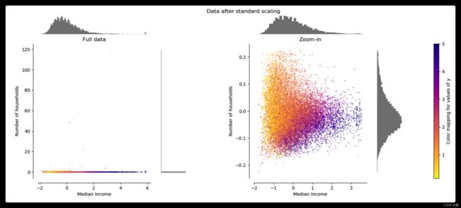
适用于:如果数据的分布本身就服从正态分布,就可以用这个方法。
通常这种方法基本可用于有outlier的情况,但是,在计算方差和均值的时候outliers仍然会影响计算。所以,在出现outliers的情况下可能会出现转换后的数的不同feature分布完全不同的情况。
如上图,经过StandardScaler之后,横坐标与纵坐标的分布出现了很大的差异,这可能是outliers造成的。
5.5、转换流水线
5.5.1、数值属性的流水线(Scikit-Learn:Pipeline)
正如你所见,许多数据转换的步骤需要以正确的顺序来执行。而Scikit-Learn正好提供了Pipeline类来支持这样的转换。下面是一个数值属性的流水线示例:
from sklearn.pipeline import Pipeline
from sklearn.preprocessing import StandardScaler

num_pipeline = Pipeline([
    ('imputer', SimpleImputer(strategy="median")),
    ('attribs_adder', CombinedAttributesAdder()),
    ('std_scaler', StandardScaler()),
])
housing_num_tr = num_pipeline.fit_transform(housing_num)
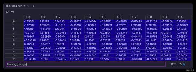
Pipeline构造函数会通过一系列名称/估值器的配对来定义步骤序列。除了最后一个是估值器之外,前面都必须是转换器(也就是说,必须有fit_transform()方法)。至于命名可以随意(只要他们是独一无二的,不含双下划线),它们稍后在超参数调整中会有用。
当调用流水线的fit()方法时,会在所有转换器上按照顺序依次调用fit_transform(),将一个调用的输出作为参数传递给下一个调用的方法,直到传递到最终的估值器,则只会调用fit()方法。
流水线的方法和最终的估值器的方法相同。在本例中,最后一个估值器是StandardScaler,这是一个转换器,因此流水线有一个transform()方法,可以按顺序将所有的转换应用到数据中(这也是我们用过的fit_transform()方法)。
5.5.2、所有属性的流水线(Scikit-Learn:ColumnTransformer)
到目前为止,我们分别处理了类别列和数值列。拥有一个能够处理所有列的转换器会更方便,将适当的转换应用于每一列。Scikit-Learn为此引入了ColumnTransformer,好消息是它与Pandas DataFrames一起使用时效果很好。让我们来用它将所有转换应用到房屋数据:
from sklearn.compose import ColumnTransformer

num_attribs = list(housing_num) # 获取列头
cat_attribs = ["ocean_proximity"]

full_pipeline = ColumnTransformer([
    ("num", num_pipeline, num_attribs),
    ("cat", OneHotEncoder(), cat_attribs),
])
housing_prepared = full_pipeline.fit_transform(housing)
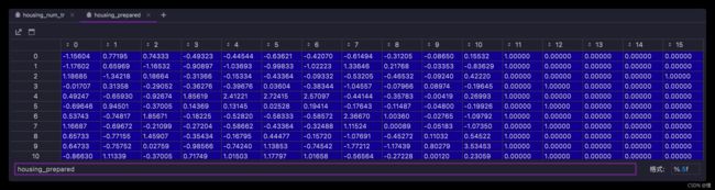
首先导入ColumnTransformer类,接下来获得数值列和类别列名称列表,然后构造一个ColumnTransformer。构造函数需要一个元组列表,其中每个元组都包含一个名称(与流水线一样)、一个转换器,以及一个该转换器能够应用的列名称(或索引)的列表。在此示例中,我们指定数值列使用之前定义的num_pipeline进行转换,类别列使用OneHotEncoder进行转换。最后,我们将ColumnTransformer应用到房屋数据:它将每个转换器应用于适当的列,并沿第二个轴合并输出(转换器必须返回相同数据的行)。
请注意,OneHotEncoder返回一个稀疏矩阵,而num_pipeline返回一个密集矩阵。当稀疏矩阵和密集矩阵混合在一起时,ColumnTransformer会估算最终矩阵的密度(即单元格的非零比率),如果密度低于给定的阈值,则返回一个稀疏矩阵(通过默认值为sparse_threshold = 0.3)。在此示例中,返回一个密集矩阵。我们有一个预处理流水线,该流水线可以获取全部房屋数据并对每一列进行适当的转换。
6、选择和训练模型
6.1、训练和评估训练集
6.1.1、LinearRegression 线性回归模型
首先,我们先训练一个线性回归模型:
from sklearn.linear_model import LinearRegression

lin_reg = LinearRegression()
lin_reg.fit(housing_prepared, housing_labels)
LinearRegression()
现在你有一个可以工作的线性回归模型了,让我们用几个训练集的实例试试:
some_data = housing[:5] # 获取前5行数据
some_labels = housing_labels.iloc[:5] # 获取前5行标签,用于验证模型结果
some_data_prepared = full_pipeline.transform(some_data) # 流水线处理数据
print("Predictions:", lin_reg.predict(some_data_prepared)) # 模型预测数据
print("Labels:", list(some_labels)) # 真实结果
Predictions: [210644.60459286 317768.80697211 210956.43331178  59218.98886849 189747.55849879]
Labels: [286600.0, 340600.0, 196900.0, 46300.0, 254500.0]
可以工作了,虽然预测还不是很准确(实际上。。。一点都不准。。。)。我们可以使用Scikit-Learn的mean_squared_error()函数来测量整个训练集上回归模型的RMSE(均方根误差):
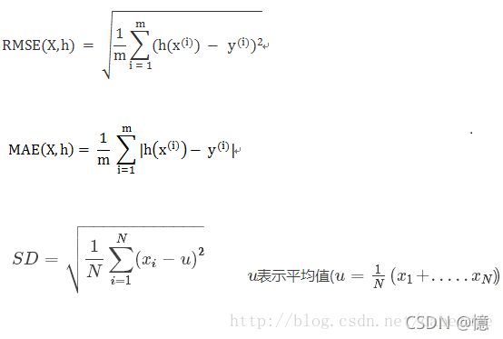
RMSE
- Root Mean Square Error,均方根误差
- 是观测值与真值偏差的平方和与观测次数m比值的平方根。
- 是用来衡量观测值同真值之间的偏差
MAE
- Mean Absolute Error ,平均绝对误差
- 是绝对误差的平均值
- 能更好地反映预测值误差的实际情况.
SD
- Standard Deviation ,标准差
- 是方差的算数平方根
- 是用来衡量一组数自身的离散程度
from sklearn.metrics import mean_squared_error

housing_predictions = lin_reg.predict(housing_prepared) # 使用模型获取训练集全部预测数据
lin_mse = mean_squared_error(housing_labels, housing_predictions) # 真实数据 与 模型预测数据 的 均方根误差
lin_rmse = np.sqrt(lin_mse) # 平方根,预测误差值
lin_rmse
68628.19819848922
median_housing_values分布在 120000~265000 美元之间,所以典型的预测误差达到 68628 美元只能说明差强人意。
这就是一个典型的模型对训练数据欠拟合的案例。这种情况发生时,通常意味着这些:
- 特征可能无法提供足够的信息来做出更好的预测;
- 或者是模型本身不够强大。
想要修正欠拟合,可以通过:
- 选择更强大的模型;
- 或为算法训练提供更好的特征;
- 又或者减少模型的限制等方法。
我们这个模型不是一个正则化的模型,所以可以排除最后一个选项。你可以尝试添加更多的特征(比如,人口数量的日志),但首选,让我们尝试一个更复杂的模型,看看它到底是怎样工作的。
6.1.2、DecisionTreeRegressor 决策树模型
我们来训练一个DecisionTreeRegressor。这是一个非常强大的模型,它能够从数据中找到复杂的非线性关系。使用方法与上面的线性回归模型相同:
from sklearn.tree import DecisionTreeRegressor

tree_reg = DecisionTreeRegressor()
tree_reg.fit(housing_prepared, housing_labels)
DecisionTreeRegressor()
训练集评估结果
housing_predictions = tree_reg.predict(housing_prepared)
tree_mse = mean_squared_error(housing_labels, housing_predictions)
tree_rmse = np.sqrt(tree_mse)
print(tree_rmse)
0.0
结果是0,没有预测误差,这个模型真的可以做到绝对完美么?当然,更可能是这个模型对数据严重过拟合了。我们应该怎么确认?前面提到过,在你有信心启动模型之前,都不要触碰测试集。
所有这里,你需要那训练集中的一部分用于训练,另一部分用于模型验证。
6.1.2.1、使用交叉验证来更好地进行评估
评估决策树模型的一种方法是使用train_test_split函数将训练集分为较小的训练集和验证集,然后根据这些较小的训练集来训练模型,并对其进行评估。这虽然有一些工作量,但是也不会太难,并且非常有效。
另一个不错的选择市使用Scikit-Learn的K-折交叉验证功能。以下是执行K-折交叉验证的代码:
- 它将训练集随机分割成10个不同的子集,每个子集称为一个折叠;
- 对决策树模型进行10次训练和评估 – 每次挑选1个折叠进行评估,使用另外的9个折叠进行训练;
- 产生的结果是一个包含10次评估分数的数组。
def display_scores(scores):
    print("分  数:", scores)
    print("平均值:", scores.mean())
    print("标准差:", scores.std())
from sklearn.model_selection import cross_val_score

# neg_mean_squared_error: 负均方误差
scores = cross_val_score(tree_reg, housing_prepared, housing_labels,
                         scoring="neg_mean_squared_error", cv=10)
tree_rmse_scores = np.sqrt(-scores)
display_scores(tree_rmse_scores)
分  数: [70062.5222628  66736.98017719 70439.6047592  70474.78239772 71238.21621992
        74620.75350778 71398.18416741 70620.80936843 77492.84330946 71004.28109473]
平均值: 71408.89772646272
标准差: 2712.8600596563356
Scikit-Learn的K-折交叉验证功能更倾向于使用效用函数(越大越好)而不是成本函数(越小越好),所以计算分数的函数实际上负的MSE(一个负值)函数,这就是为什么上面的代码在计算平方根之前会先计算出-scores。
这次的决策树模型好像不如之前的表现得好,事实上,它看起来简直比线性回归模型还要糟糕。请注意,交叉验证不仅可以得到一个模型性能的评估值,还可以衡量该评估的精准度(即其标准差)。这里该决策树得到的评分约为71407,上下浮动±2439。如果你只使用了一个验证集,就收不到这样的结果信息。交叉验证的代价就是要多次训练模型,因此也不是永远都行得通。
保险起见,让我们也计算一下线性回归模型的评分:
lin_scores = cross_val_score(lin_reg, housing_prepared, housing_labels,
                             scoring="neg_mean_squared_error", cv=10)
lin_rmse_scores = np.sqrt(-lin_scores)
display_scores(lin_rmse_scores)
分  数: [66782.73843989 66960.118071 70347.95244419 74739.57052552 68031.13388938
        71193.84183426 64969.63056405 68281.61137997 71552.91566558 67665.10082067]
平均值: 69052.46136345083
标准差: 2731.674001798347
没错,决策树模型的确严重过拟合了,以至于表现得比线性回归模型还要糟糕。
6.1.3、RndomForestRegressor 随机森林模型
我们再来试试最后一个模型RndomForestRegressor。随机森林的工作原理:通过对特征的随机子集进行许多个决策树的训练,然后对其预测取平均。在多个模型的基础之上建立模型,称之为集成学习,这是进一步推动机器学习算法的好方法。这里我们将跳过大部分代码,因为与其他模型基本相同:
from sklearn.ensemble import RandomForestRegressor

forest_reg = RandomForestRegressor()
forest_reg.fit(housing_prepared, housing_labels)
RandomForestRegressor()
housing_predictions = forest_reg.predict(housing_prepared)
forest_mse = mean_squared_error(housing_labels, housing_predictions)
forest_rmse = np.sqrt(forest_mse)
print(forest_rmse)
18725.06655956781
forest_scores = cross_val_score(forest_reg, housing_prepared, housing_labels,
                                scoring="neg_mean_squared_error", cv=10)
forest_rmse_scores = np.sqrt(-forest_scores)
display_scores(forest_rmse_scores)
分  数: [49809.66295035 47362.11725625 50097.32716715 51971.44001152 49498.75378409
        53481.17484005 49051.91408781 48402.93749135 52812.15210493 50385.42811085]
平均值: 50287.290780434654
标准差: 1842.3191312235808
当前数据看起来是目前对好的。但是,请注意,训练集上的分数(18725)仍然远低于验证集(50287),这意味着该模型仍然对训练集过拟合。过拟合的可能解决方案包括:
- 简化模型
- 约束模型(即使其正规化)
- 或获得更多的训练数据
不过在深入探索随机森林之前,你应该先尝试一遍各种机器学习算法的其他模型(几种具有不同内核的支持向量机,比如神经网络模型等),但记住,别花太多时间去调整超参数,我们的目的是筛选出几个(2~5个)有效的模型。
每一个尝试过的模型都应该妥善的保存,以便将来可以轻松回顾。通过
Python的pickle模块或joblib库,你可以轻松保存Scikit-Learn模型,这样可以更有效地将大型NumPy数组序列号。
7、微调模型
假设你现在有了一个有效模型的候选列表。现在你需要对它们进行微调。我们来看几个可行的方法。
7.1、网格搜索
一种微调的方式是以手动调整超参数,直到找到一组很好的超参数组合。这个过程非常枯燥乏味,你可以坚持不到足够的时间来探索出各种组合。
相反,你可以用Scikit-Learn的GridSearchCV来替你进行探索。你所需要做的只是告诉它你要进行实验的超参数是什么,以及需要尝试的值,它将会使用交叉验证来评估超参数的所有可能组合。例如,下面这段代码搜索RandomForestRegressor的超参数数值的最佳组:
from sklearn.model_selection import GridSearchCV

param_grid = [
    {
     "n_estimators": [3, 10, 30], "max_features": [2, 4, 6, 8]},
    {
     "bootstrap": [False], "n_estimators": [3, 10], "max_features": [2, 3, 4]},
]
forest_reg = RandomForestRegressor()
grid_search = GridSearchCV(forest_reg, param_grid, cv=5,
                           scoring="neg_mean_squared_error",
                           return_train_score=True)
grid_search.fit(housing_prepared, housing_labels)
GridSearchCV(cv=5, estimator=RandomForestRegressor(),
             param_grid=[{'max_features': [2, 4, 6, 8],
                          'n_estimators': [3, 10, 30]},
                         {'bootstrap': [False], 'max_features': [2, 3, 4],
                          'n_estimators': [3, 10]}],
             return_train_score=True, scoring='neg_mean_squared_error')
当你不知道超参数应该赋什么值时,一个简单的方法是尝试10次连续幂次方(如果你想要得到更细粒度的搜索,可以使用更小的数,参考这个示例中
n_estimators超参数。
这个param_grid告诉Scikit-Learn,首先评估第一个dict中的n_estimators和max_features的所有 3×4=12 种超参数组合;接着,尝试第二个dict中超参数的所有 1×2×3=6 种组合,但这次超参数bootstrap需要设置为False而不是True。
总而言之,网格探索将探索RandomForestRegressor超参数值的 12+6=18 种组合,并对每个模型进行5次训练(cv=5)。换句话,总共完成 18×5=90 次训练。
但是训练完成后你就可以获得最佳的参数组合:
grid_search.best_params_
{'max_features': 6, 'n_estimators': 30}
你可以直接得到最好的估算器:
grid_search.best_estimator_
RandomForestRegressor(max_features=6, n_estimators=30)
如果GridSearchCV被初始化为refit=True(默认值),那么一旦通过交叉验证找到最佳估算器,它将在整个训练集上重新训练。这通常是个好方法,因为提供更多的数据很可能提升其性能。
当然还有评估分数:
cvres = grid_search.cv_results_
for mean_score, params in zip(cvres["mean_test_score"], cvres["params"]):
    print(np.sqrt(-mean_score), params)
64219.37103342171 {'max_features': 2, 'n_estimators': 3}
55757.44574868692 {'max_features': 2, 'n_estimators': 10}
52912.46028198916 {'max_features': 2, 'n_estimators': 30}
60369.36943060073 {'max_features': 4, 'n_estimators': 3}
53342.610401252685 {'max_features': 4, 'n_estimators': 10}
50755.23490862702 {'max_features': 4, 'n_estimators': 30}
59396.83436658384 {'max_features': 6, 'n_estimators': 3}
52375.46588717245 {'max_features': 6, 'n_estimators': 10}
50133.101632717895 {'max_features': 6, 'n_estimators': 30}
58851.03261455543 {'max_features': 8, 'n_estimators': 3}
52154.38996091269 {'max_features': 8, 'n_estimators': 10}
50142.71940679718 {'max_features': 8, 'n_estimators': 30}
63061.98058118926 {'bootstrap': False, 'max_features': 2, 'n_estimators': 3}
54457.63242342584 {'bootstrap': False, 'max_features': 2, 'n_estimators': 10}
59490.18437223276 {'bootstrap': False, 'max_features': 3, 'n_estimators': 3}
52951.47441756218 {'bootstrap': False, 'max_features': 3, 'n_estimators': 10}
59440.60460822187 {'bootstrap': False, 'max_features': 4, 'n_estimators': 3}
51717.31614272946 {'bootstrap': False, 'max_features': 4, 'n_estimators': 10}
在本例中,我们得到的最佳解决方案是将超参数max_features设置为6,n_estimators设置为30。这个组合的RMSE分数为50133,略优于之前默认参数的分数50287。
7.2、随机搜索
如果探索的组合数量太少(例如上一个案例),那么网格搜索是一个不错的方法。但是当超参数的搜索范围比较大时,通过会优先选择使用RandomizedSearchCV。这个类用起来与GridSearchCV类大致相同,但是它不会尝试所有可能的组合,而是在每次迭代中为每个超参数选择一个随机值,然后对一定数量的随机组合进行评估。这种方法有两个显著好处:
- 如果运行随机搜索1000个迭代,那么将会探索每个超参数的1000个不同的值。
- 通过简单的设置迭代次数,可以更好地控制要分配给超参数搜索的计算预算。
from sklearn.model_selection import RandomizedSearchCV
from scipy.stats import randint

param_distribs = {

    'n_estimators': randint(low=1, high=200),
    'max_features': randint(low=1, high=8),
}

forest_reg = RandomForestRegressor()
rnd_search = RandomizedSearchCV(forest_reg, param_distributions=param_distribs,
                                n_iter=10, cv=5, scoring='neg_mean_squared_error')
rnd_search.fit(housing_prepared, housing_labels)
RandomizedSearchCV(cv=5, estimator=RandomForestRegressor(),
                   param_distributions={'max_features': ,
                                        'n_estimators': },
                   scoring='neg_mean_squared_error')
cvres = rnd_search.cv_results_
for mean_score, params in zip(cvres["mean_test_score"], cvres["params"]):
    print(np.sqrt(-mean_score), params)
49182.98287156724 {'max_features': 6, 'n_estimators': 142}
49256.64243951438 {'max_features': 7, 'n_estimators': 157}
49705.21035567195 {'max_features': 7, 'n_estimators': 59}
68431.80112151649 {'max_features': 1, 'n_estimators': 3}
49547.2056799527 {'max_features': 4, 'n_estimators': 144}
51481.190769293426 {'max_features': 5, 'n_estimators': 13}
59848.891702369874 {'max_features': 1, 'n_estimators': 9}
49482.15331762217 {'max_features': 4, 'n_estimators': 188}
50134.64676419512 {'max_features': 3, 'n_estimators': 162}
55151.747332409956 {'max_features': 1, 'n_estimators': 47}
7.3、集成方法
还有一种微调系统的方法是将表现最优的模型组合起来。组合(或“集成”)方法通过最佳的单一模型更好(就像随机森林比任何单个的决策树模型更好一样),特别是当单一模型会产生不同类型误差时更是如此。
7.4、分析最佳模型及其误差
通过检查最佳模型,你总是可以得到一些好的洞见。例如在进行准确预测时,RandomForestRegressor可以指出每个属性的相对重要程度:
feature_importances = grid_search.best_estimator_.feature_importances_
feature_importances
array([8.20349643e-02, 7.08313931e-02, 4.31025707e-02, 1.82135239e-02,
       1.66778827e-02, 1.83580953e-02, 1.58181207e-02, 2.93820957e-01,
       5.79152902e-02, 1.08181525e-01, 1.01867756e-01, 1.83167523e-02,
       1.43188327e-01, 4.00992699e-05, 4.73585356e-03, 6.89688957e-03])
将这些重要性分数显示在对应的属性名称旁边:
extra_attribs = ["rooms_per_hhold", "pop_per_hhold", "bedrooms_per_room"]
#cat_encoder = cat_pipeline.named_steps["cat_encoder"] # 旧版本
cat_encoder = full_pipeline.named_transformers_["cat"]
cat_one_hot_attribs = list(cat_encoder.categories_[0])
attributes = num_attribs + extra_attribs + cat_one_hot_attribs
sorted(zip(feature_importances, attributes), reverse=True)
[(0.2938209569026082, 'median_income'),
 (0.14318832667800896, 'INLAND'),
 (0.10818152506358511, 'pop_per_hhold'),
 (0.10186775584763018, 'bedrooms_per_room'),
 (0.08203496427830204, 'longitude'),
 (0.07083139305733996, 'latitude'),
 (0.057915290153382135, 'rooms_per_hhold'),
 (0.043102570688951285, 'housing_median_age'),
 (0.01835809530124593, 'population'),
 (0.018316752295000915, '<1H OCEAN'),
 (0.01821352394132179, 'total_rooms'),
 (0.0166778826835988, 'total_bedrooms'),
 (0.015818120710775083, 'households'),
 (0.006896889571023202, 'NEAR OCEAN'),
 (0.0047358535572835985, 'NEAR BAY'),
 (4.009926994286412e-05, 'ISLAND')]
7.5、通过测试集评估系统
通过一段时间的训练,你终于有了一个表现足够优秀的系统。现在是用测试集评估最终模型的时候了。这个过程没有什么特别的,只需要从测试集中获取预测器和标签,运行full_pipline来转换数据(调用transform()而不是fit_transform()),然后在测试集上评估最终模型:
final_model = rnd_search.best_estimator_

X_test = strat_test_set.drop("median_house_value", axis=1)
y_test = strat_test_set["median_house_value"].copy()

X_test_prepared = full_pipeline.transform(X_test)
final_predictions = final_model.predict(X_test_prepared)

final_mse = mean_squared_error(y_test, final_predictions)
final_rmse = np.sqrt(final_mse)
final_rmse
46979.86059266281
如果想知道这个估计的精确度。为此,你可以使用scipy.stats.t.interval()计算泛化误差的95%置信区间:
from scipy import stats

confidence = 0.95
squared_errors = (final_predictions - y_test) ** 2
np.sqrt(stats.t.interval(confidence, len(squared_errors) - 1,
                         loc=squared_errors.mean(),
                         scale=stats.sem(squared_errors)))
array([45009.06645486, 48871.24450507])
如果之前进行过大量的超参数调整,这时的评估结果通常会略逊色与之前使用的交叉验证时的表现结果(因为通过不断调整,系统在验证数据上终于表现良好,在未知数据集上可能达不到那么好的效果)。这时不要再继续调整超参数,因为这些改进在泛化到新数据集时又会变成无用功。(这里我做了上万次的超参数调整,提升不明显)
在本案例中,系统的最终性能可能并不比专家估算的效果更好,通过会下降20%左右,但是依然可以为专家腾出大量时间,投入到其他任务上。
8、上述完整关键代码总结
import os
import tarfile
import urllib.request

import pandas as pd
import numpy as np
from sklearn.model_selection import StratifiedShuffleSplit
from sklearn.impute import SimpleImputer
from sklearn.preprocessing import OneHotEncoder
from sklearn.base import BaseEstimator, TransformerMixin
from sklearn.pipeline import Pipeline
from sklearn.preprocessing import StandardScaler
from sklearn.compose import ColumnTransformer
from sklearn.linear_model import LinearRegression
from sklearn.metrics import mean_squared_error
from sklearn.tree import DecisionTreeRegressor
from sklearn.model_selection import cross_val_score
from sklearn.ensemble import RandomForestRegressor
from sklearn.model_selection import GridSearchCV
from sklearn.model_selection import RandomizedSearchCV
from scipy.stats import randint
from scipy import stats

DOWNLOAD_ROOT = "https://raw.githubusercontent.com/ageron/handson-ml2/master/"
HOUSING_PATH = os.path.join("datasets", "housing")
HOUSING_URL = DOWNLOAD_ROOT + "datasets/housing/housing.tgz"


def fetch_housing_data(housing_url=HOUSING_URL, housing_path=HOUSING_PATH):
	"""
	下载数据
	"""
    if not os.path.isdir(housing_path):
        os.makedirs(housing_path)
    tgz_path = os.path.join(housing_path, "housing.tgz")
    urllib.request.urlretrieve(housing_url, tgz_path)
    housing_tgz = tarfile.open(tgz_path)
    housing_tgz.extractall(path=housing_path)
    housing_tgz.close()


def load_housing_data(housing_path=HOUSING_PATH):
	"""
	读取数据
	"""
    csv_path = os.path.join(housing_path, "housing.csv")
    return pd.read_csv(csv_path)


# "total_rooms", "total_bedrooms", "population", "households"
rooms_ix, bedroom_ix, population_ix, households_ix = 3, 4, 5, 6


class CombinedAttributesAdder(BaseEstimator, TransformerMixin):
	"""
	自定义转换器
	"""
    def __init__(self, add_bedroom_per_room=True):
        self.add_bedroom_per_room = add_bedroom_per_room

    def fit(self, X, y=None):
        return self

    def transform(self, X):
        """
        X[:, rooms_ix]:X数组,":"所有行,取rooms_ix列的数据(即,取第rooms_ix列的全部数据,从0开始计数)
        ------------
        np.r_是按列连接两个矩阵,就是把两矩阵上下相加,要求列数相等。
        np.c_是按行连接两个矩阵,就是把两矩阵左右相加,要求行数相等。即添加计算后的新列数据
        例:
            a = np.array([[1, 2, 3],
                          [7,8,9]])
            b = np.array([[4,5,6],
                          [1,2,3]])
            c = np.c_[a,b]

            >>> print(c)
            array([[1, 2, 3, 4, 5, 6],
                   [7, 8, 9, 1, 2, 3]])
        """
        rooms_per_household = X[:, rooms_ix] / X[:, households_ix]
        population_per_household = X[:, population_ix] / X[:, households_ix]
        if self.add_bedroom_per_room:
            bedrooms_per_room = X[:, bedroom_ix] / X[:, rooms_ix]
            return np.c_[X, rooms_per_household, population_per_household, bedrooms_per_room]
        else:
            return np.c_[X, rooms_per_household, population_per_household]


def display_scores(scores):
    print("分  数:", scores)
    print("平均值:", scores.mean())
    print("标准差:", scores.std())


if __name__ == '__main__':
    # 下载数据
    fetch_housing_data()
    # 读取数据
    housing = load_housing_data()
    # 按收入分组
    housing["income_cat"] = pd.cut(housing["median_income"],
                                   bins=[0, 1.5, 3, 4.5, 6, np.inf],
                                   labels=[1, 2, 3, 4, 5])
    # 按income_cat类别比例抽取 20% 的测试集 和 80% 的训练集
    split = StratifiedShuffleSplit(n_splits=1, test_size=0.2, random_state=42)
    for train_index, test_index in split.split(housing, housing["income_cat"]):
        strat_train_set = housing.loc[train_index]
        strat_test_set = housing.loc[test_index]
    # 删除收入分组,恢复数据
    for set_ in (strat_train_set, strat_test_set):
        set_.drop("income_cat", axis=1, inplace=True)
    # 寻找数据相关性
    corr_matrix = housing.corr()
    corr_matrix["median_house_value"].sort_values(ascending=False)
    """
    数据处理:
        1、训练集拆分成 预测集(housing)和标签(housing_labels);
        2、预测集再拆分出 数字属性(housing_num)和 文本属性(ocean_proximity)
    """
    housing = strat_train_set.drop("median_house_value", axis=1)
    housing_labels = strat_train_set["median_house_value"].copy()
    housing_num = housing.drop("ocean_proximity", axis=1)
    """
    数值属性流水线:
        1、SimpleImputer(中位数填充缺失值);
        2、CombinedAttributesAdder(自定义转化器);
        3、StandardScaler(特征缩放)
    """
    num_pipeline = Pipeline([
        ('imputer', SimpleImputer(strategy="median")),
        ('attribs_adder', CombinedAttributesAdder()),
        ('std_scaler', StandardScaler()),
    ])
    housing_num_tr = num_pipeline.fit_transform(housing_num)

    num_attribs = list(housing_num)  # 获取数字集列头列表
    cat_attribs = ["ocean_proximity"]
    """
    所有属性的流水线:
        1、num_pipeline(数值属性流水线);
        2、OneHotEncoder(文本属性 转换为 独热向量)
    """
    full_pipeline = ColumnTransformer([
        ("num", num_pipeline, num_attribs),
        ("cat", OneHotEncoder(), cat_attribs),
    ])
    housing_prepared = full_pipeline.fit_transform(housing)

    print("********************* 线性回归模型 *********************")
    # 线性回归模型
    lin_reg = LinearRegression()
    lin_reg.fit(housing_prepared, housing_labels)
    housing_predictions = lin_reg.predict(housing_prepared)
    lin_mse = mean_squared_error(housing_labels, housing_predictions)
    lin_rmse = np.sqrt(lin_mse)
    print(lin_rmse)
    # K-交叉验证 - 线性回归模型
    lin_scores = cross_val_score(lin_reg, housing_prepared, housing_labels, scoring="neg_mean_squared_error", cv=10)
    lin_rmse_scores = np.sqrt(-lin_scores)
    display_scores(lin_rmse_scores)

    print("********************* 决策树模型 *********************")
    # 决策树模型
    tree_reg = DecisionTreeRegressor()
    tree_reg.fit(housing_prepared, housing_labels)
    housing_predictions = tree_reg.predict(housing_prepared)
    tree_mse = mean_squared_error(housing_labels, housing_predictions)
    tree_rmse = np.sqrt(tree_mse)
    print(tree_rmse)
    # K-交叉验证 - 决策树模型
    scores = cross_val_score(tree_reg, housing_prepared, housing_labels, scoring="neg_mean_squared_error", cv=10)
    tree_rmse_scores = np.sqrt(-scores)
    display_scores(tree_rmse_scores)

    print("********************* 随机森林模型 *********************")
    # 随机森林模型
    forest_reg = RandomForestRegressor()
    forest_reg.fit(housing_prepared, housing_labels)
    housing_predictions = forest_reg.predict(housing_prepared)
    forest_mse = mean_squared_error(housing_labels, housing_predictions)
    forest_rmse = np.sqrt(forest_mse)
    print(forest_rmse)
    # K-交叉验证 - 随机森林模型
    forest_scores = cross_val_score(forest_reg, housing_prepared, housing_labels, scoring="neg_mean_squared_error", cv=10)
    forest_rmse_scores = np.sqrt(-forest_scores)
    display_scores(forest_rmse_scores)

    print("********************* 超参数微调 随机森林模型 网格搜索 *********************")
    """
    模型参数微调:
        模型:随机森林模型
        方法:网格搜索
    """
    param_grid = [
        {
     "n_estimators": [3, 10, 30], "max_features": [2, 4, 6, 8]},
        {
     "bootstrap": [False], "n_estimators": [3, 10], "max_features": [2, 3, 4]},
    ]
    forest_reg = RandomForestRegressor()
    grid_search = GridSearchCV(forest_reg, param_grid, cv=5, scoring="neg_mean_squared_error", return_train_score=True)
    grid_search.fit(housing_prepared, housing_labels)
    # 微调结果
    cvres = grid_search.cv_results_
    for mean_score, params in zip(cvres["mean_test_score"], cvres["params"]):
        print(np.sqrt(-mean_score), params)

    print("********************* 超参数微调 随机森林模型 随机搜索 *********************")
    """
    模型参数微调:
        模型:随机森林模型
        方法:随机搜索
    """
    param_distribs = {

        'n_estimators': randint(low=1, high=200),
        'max_features': randint(low=1, high=8),
    }
    forest_reg = RandomForestRegressor()
    rnd_search = RandomizedSearchCV(forest_reg, param_distributions=param_distribs,
                                    n_iter=10, cv=5, scoring='neg_mean_squared_error')
    rnd_search.fit(housing_prepared, housing_labels)
    # 微调结果
    cvres = rnd_search.cv_results_
    for mean_score, params in zip(cvres["mean_test_score"], cvres["params"]):
        print(np.sqrt(-mean_score), params)

    print("********************* 随机森林最优模型 测试集评估系统 *********************")
    final_model = rnd_search.best_estimator_

    X_test = strat_test_set.drop("median_house_value", axis=1)
    y_test = strat_test_set["median_house_value"].copy()

    X_test_prepared = full_pipeline.transform(X_test)
    final_predictions = final_model.predict(X_test_prepared)

    final_mse = mean_squared_error(y_test, final_predictions)
    final_rmse = np.sqrt(final_mse)
    print(final_rmse)
    # 评估的精确度,计算泛化误差的95%置信区间:
    confidence = 0.95
    squared_errors = (final_predictions - y_test) ** 2
    np.sqrt(stats.t.interval(confidence, len(squared_errors) - 1,
                             loc=squared_errors.mean(),
                             scale=stats.sem(squared_errors)))