动手学习深度学习-深度学习基础
本文章仅为本人在学习过程中的记录笔记,如有侵权,请联系。
李沐大神的课程地址:https://courses.d2l.ai/zh-v2/
3.20课程
深度学习介绍:


数据操作
首先,我们导入 torch。
import torch
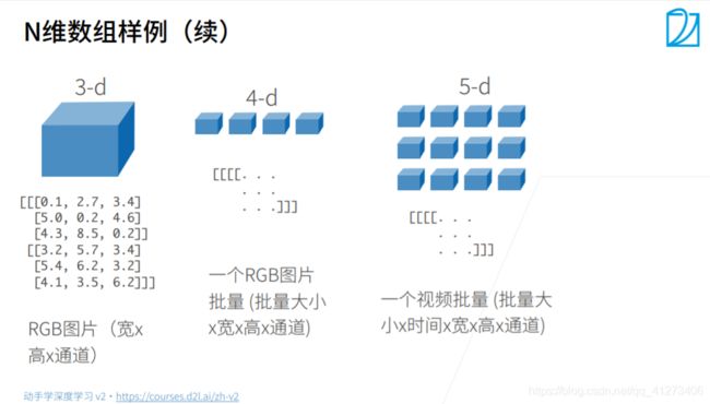
张量表示一个数值组成的数组,这个数组可能有多个维度
x = torch.arange(12)
x
tensor([ 0, 1, 2, 3, 4, 5, 6, 7, 8, 9, 10, 11])
我们可以通过张量的 shape 属性来访问张量的 形状 和张量中元素的总数
x.shape
torch.Size([12])
x.numel()
12
要改变一个张量的形状而不改变元素数量和元素值,我们可以调用 reshape 函数。
x = x.reshape(3, 4)
x
tensor([[ 0,  1,  2,  3],
        [ 4,  5,  6,  7],
        [ 8,  9, 10, 11]])
使用全0、全1、其他常量或者从特定分布中随机采样的数字
torch.zeros((2, 3, 4))
tensor([[[0., 0., 0., 0.],
         [0., 0., 0., 0.],
         [0., 0., 0., 0.]],

        [[0., 0., 0., 0.],
         [0., 0., 0., 0.],
         [0., 0., 0., 0.]]])
torch.ones((2, 3, 4))
tensor([[[1., 1., 1., 1.],
         [1., 1., 1., 1.],
         [1., 1., 1., 1.]],

        [[1., 1., 1., 1.],
         [1., 1., 1., 1.],
         [1., 1., 1., 1.]]])
torch.randn(3, 4)
tensor([[ 1.5592,  0.7887, -1.0770, -0.2182],
        [ 0.6342, -0.7517, -0.0655,  0.3767],
        [ 0.3668, -1.3558, -0.4728, -0.6023]])
通过提供包含数值的 Python 列表(或嵌套列表)来为所需张量中的每个元素赋予确定值
torch.tensor([[2, 1, 4, 3], [1, 2, 3, 4], [4, 3, 2, 1]]).shape
torch.Size([3, 4])
常见的标准算术运算符(+、-、*、/ 和 **)都可以被升级为按元素运算:
x = torch.tensor([1.0, 2, 4, 8])
y = torch.tensor([2, 2, 2, 2])
x + y, x - y, x * y, x / y, x**y
(tensor([ 3.,  4.,  6., 10.]),
 tensor([-1.,  0.,  2.,  6.]),
 tensor([ 2.,  4.,  8., 16.]),
 tensor([0.5000, 1.0000, 2.0000, 4.0000]),
 tensor([ 1.,  4., 16., 64.]))
按按元素方式应用更多的计算:
torch.exp(x)
tensor([2.7183e+00, 7.3891e+00, 5.4598e+01, 2.9810e+03])
我们也可以把多个张量连结在一起
x = torch.arange(12, dtype=torch.float32).reshape((3, 4))
y = torch.tensor([[2.0, 1, 4, 3], [1, 2, 3, 4], [4, 3, 2, 1]])
torch.cat((x, y), dim=0), torch.cat((x, y), dim=1)
(tensor([[ 0.,  1.,  2.,  3.],
         [ 4.,  5.,  6.,  7.],
         [ 8.,  9., 10., 11.],
         [ 2.,  1.,  4.,  3.],
         [ 1.,  2.,  3.,  4.],
         [ 4.,  3.,  2.,  1.]]),
 tensor([[ 0.,  1.,  2.,  3.,  2.,  1.,  4.,  3.],
         [ 4.,  5.,  6.,  7.,  1.,  2.,  3.,  4.],
         [ 8.,  9., 10., 11.,  4.,  3.,  2.,  1.]]))
通过 逻辑运算符 构建二元张量
print(x,'\n', y)
x == y
tensor([[ 0.,  1.,  2.,  3.],
        [ 4.,  5.,  6.,  7.],
        [ 8.,  9., 10., 11.]])
 tensor([[2., 1., 4., 3.],
        [1., 2., 3., 4.],
        [4., 3., 2., 1.]])


tensor([[False,  True, False,  True],
        [False, False, False, False],
        [False, False, False, False]])
对张量中的所有元素进行求和会产生一个只有一个元素的张量。
x.sum()
tensor(66.)
即使形状不同,我们仍然可以通过调用 广播机制 (broadcasting mechanism) 来执行按元素操作
a = torch.arange(3).reshape((3, 1))
b = torch.arange(2).reshape((1, 2))
a, b
(tensor([[0],
         [1],
         [2]]),
 tensor([[0, 1]]))
a + b
tensor([[0, 1],
        [1, 2],
        [2, 3]])
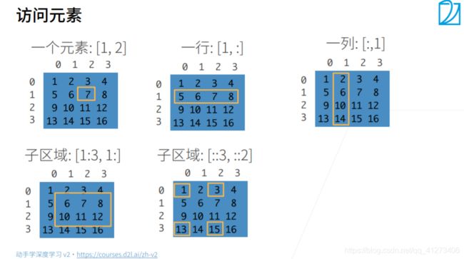
可以用 [-1] 选择最后一个元素,可以用 [1:3] 选择第二个和第三个元素`
x[-1], x[1:3]
(tensor([ 8.,  9., 10., 11.]),
 tensor([[ 4.,  5.,  6.,  7.],
         [ 8.,  9., 10., 11.]]))
除读取外,我们还可以通过指定索引来将元素写入矩阵。
print(x)
x[1, 2] = 9
print(x)
tensor([[ 0.,  1.,  2.,  3.],
        [ 4.,  5.,  6.,  7.],
        [ 8.,  9., 10., 11.]])
tensor([[ 0.,  1.,  2.,  3.],
        [ 4.,  5.,  9.,  7.],
        [ 8.,  9., 10., 11.]])
为多个元素赋值相同的值,我们只需要索引所有元素,然后为它们赋值。
x[0:2, :] = 12
print(x)
tensor([[12., 12., 12., 12.],
        [12., 12., 12., 12.],
        [ 8.,  9., 10., 11.]])
tensor([[12., 12., 12., 12.],
        [12., 12., 12., 12.],
        [ 8.,  9., 10., 11.]])
运行一些操作可能会导致为新结果分配内存
before = id(y) # id 内存地址
y = y + x
id(y) == before
False
执行原地操作
z = torch.zeros_like(y)
print('id(z):', id(z))
z[:] = x + y
print('id(z):', id(z))
id(z): 2029580244960
id(z): 2029580244960
如果在后续计算中没有重复使用 X,我们也可以使用 X[:] = X + Y 或 X += Y 来减少操作的内存开销。
before = id(x)
x += y
id(x) == before
True
转换为 NumPy 张量
a =  x.numpy()
b = torch.tensor(a)

type(a), type(b)
(numpy.ndarray, torch.Tensor)
将大小为1的张量转换为 Python 标量
a = torch.tensor([3.5])
a, a.item(), float(a), int(a)
(tensor([3.5000]), 3.5, 3.5, 3)
数据预处理

创建一个人工数据集,并存储在csv(逗号分隔值)文件
import os

os.makedirs(os.path.join('..', 'data'), exist_ok=True)
data_file = os.path.join('..', 'data', 'house_tiny.csv')
with open(data_file, 'w') as f:
    f.write('NumRooms,Alley,Price\n')  # 列名
    f.write('NA,Pave,127500\n')  # 每行表示一个数据样本 NA:未知数
    f.write('2,NA,106000\n')
    f.write('4,NA,178100\n')
    f.write('NA,NA,140000\n')
import pandas as pd

data = pd.read_csv(data_file)#读取csv文件
print(data)
data
   NumRooms Alley   Price
0       NaN  Pave  127500
1       2.0   NaN  106000
2       4.0   NaN  178100
3       NaN   NaN  140000
| NumRooms | Alley | Price | |
|---|---|---|---|
| 0 | NaN | Pave | 127500 |
| 1 | 2.0 | NaN | 106000 |
| 2 | 4.0 | NaN | 178100 |
| 3 | NaN | NaN | 140000 |
为了处理缺失的数据,典型的方法包括 插值 和 删除, 这里,我们将考虑插值
inputs, outputs = data.iloc[:, 0:2], data.iloc[:, 2] # 将数据切分成两部分
print(inputs,'\n',outputs)
inputs = inputs.fillna(inputs.mean())

print(inputs)
   NumRooms Alley
0       NaN  Pave
1       2.0   NaN
2       4.0   NaN
3       NaN   NaN
 0    127500
1    106000
2    178100
3    140000
Name: Price, dtype: int64
   NumRooms Alley
0       3.0  Pave
1       2.0   NaN
2       4.0   NaN
3       3.0   NaN
对于 inputs 中的类别值或离散值,我们将 “NaN” 视为一个类别。
inputs = pd.get_dummies(inputs, dummy_na=True) #one-hot编码
print(inputs)
   NumRooms  Alley_Pave  Alley_nan
0       3.0           1          0
1       2.0           0          1
2       4.0           0          1
3       3.0           0          1
现在 inputs 和 outputs 中的所有条目都是数值类型,它们可以转换为张量格式:
import torch

x, y = torch.tensor(inputs.values), torch.tensor(outputs.values)
x, y
(tensor([[3., 1., 0.],
         [2., 0., 1.],
         [4., 0., 1.],
         [3., 0., 1.]], dtype=torch.float64),
 tensor([127500, 106000, 178100, 140000]))
reshape与view:
a = torch.arange(12)
b = a.reshape((3, 4))
print(a)
b[:]=2
print(a)
tensor([ 0,  1,  2,  3,  4,  5,  6,  7,  8,  9, 10, 11])
tensor([2, 2, 2, 2, 2, 2, 2, 2, 2, 2, 2, 2])
a = torch.arange(12)
b = a.view((3, 4))
print(a)
b[:]=2
print(a)
tensor([ 0,  1,  2,  3,  4,  5,  6,  7,  8,  9, 10, 11])
tensor([2, 2, 2, 2, 2, 2, 2, 2, 2, 2, 2, 2])
3.21课程
线性代数
标量由只有一个元素的张量表示
import torch

x = torch.tensor([3.0])
y = torch.tensor([2.0])

x + y, x * y, x/y, x**y
(tensor([5.]), tensor([6.]), tensor([1.5000]), tensor([9.]))
可以将向量视为标量值组成的列表:
x = torch.arange(4)
x
tensor([0, 1, 2, 3])
通过张量的索引来访问任一元素:
x[3]
tensor(3)
访问张量的长度:
len(x)
4
只有一个轴的张量,形状只有一个元素:
x.shape
torch.Size([4])
通过指定两个分量m 和 n来创建一个形状为m×n 的矩阵:
a = torch.arange(20).reshape((5, 4))
a
tensor([[ 0,  1,  2,  3],
        [ 4,  5,  6,  7],
        [ 8,  9, 10, 11],
        [12, 13, 14, 15],
        [16, 17, 18, 19]])
矩阵的转置:
a.T
tensor([[ 0,  4,  8, 12, 16],
        [ 1,  5,  9, 13, 17],
        [ 2,  6, 10, 14, 18],
        [ 3,  7, 11, 15, 19]])
对称矩阵(symmetric matrix) A 等于其转置:A= A ⊤ A^⊤ A⊤
b = torch.tensor([[1, 2, 3], [2, 0, 4], [3, 4, 5]])
b
tensor([[1, 2, 3],
        [2, 0, 4],
        [3, 4, 5]])
b == b.T
tensor([[True, True, True],
        [True, True, True],
        [True, True, True]])
就像向量是标量的推广,矩阵是向量的推广一样,我们可以构建具有更多轴的数据结构:
x = torch.arange(24).reshape((2, 3, 4))
x
tensor([[[ 0,  1,  2,  3],
         [ 4,  5,  6,  7],
         [ 8,  9, 10, 11]],

        [[12, 13, 14, 15],
         [16, 17, 18, 19],
         [20, 21, 22, 23]]])
给定具有相同形状的任何两个张量,任何按元素二元运算的结果都将是相同形状的张量:
A = torch.arange(20, dtype=torch.float32).reshape(5, 4)
B = A.clone() # 通过分配新的内存, 将A的一个副本分配给B

A , A + B
(tensor([[ 0.,  1.,  2.,  3.],
         [ 4.,  5.,  6.,  7.],
         [ 8.,  9., 10., 11.],
         [12., 13., 14., 15.],
         [16., 17., 18., 19.]]),
 tensor([[ 0.,  2.,  4.,  6.],
         [ 8., 10., 12., 14.],
         [16., 18., 20., 22.],
         [24., 26., 28., 30.],
         [32., 34., 36., 38.]]))
两个矩阵的按元素乘法称为 哈达玛积(Hadamard product)(数学符号 ⊙):
A * B
tensor([[  0.,   1.,   4.,   9.],
        [ 16.,  25.,  36.,  49.],
        [ 64.,  81., 100., 121.],
        [144., 169., 196., 225.],
        [256., 289., 324., 361.]])
a = 2
X = torch.arange(24).reshape(2, 3, 4)
a + X , (a * X).shape
(tensor([[[ 2,  3,  4,  5],
          [ 6,  7,  8,  9],
          [10, 11, 12, 13]],

         [[14, 15, 16, 17],
          [18, 19, 20, 21],
          [22, 23, 24, 25]]]),
 torch.Size([2, 3, 4]))
计算其元素的和
x  = torch.arange(4, dtype=torch.float32)
x, x.sum()
(tensor([0., 1., 2., 3.]), tensor(6.))
表示任意形状张量的元素和
print(A)
A.shape, A.sum()
tensor([[ 0.,  1.,  2.,  3.],
        [ 4.,  5.,  6.,  7.],
        [ 8.,  9., 10., 11.],
        [12., 13., 14., 15.],
        [16., 17., 18., 19.]])


(torch.Size([5, 4]), tensor(190.))
指定求和汇总张量的轴
A_sum_axis0 = A.sum(axis=0)#axis=0 计算列
A_sum_axis0, A_sum_axis0.shape
(tensor([40., 45., 50., 55.]), torch.Size([4]))
A_sum_axis1 = A.sum(axis=1)#axis=1 计算行
A_sum_axis1, A_sum_axis1.shape
(tensor([ 6., 22., 38., 54., 70.]), torch.Size([5]))
A.sum(), A.sum(axis=[0,1])
(tensor(190.), tensor(190.))
一个与求和相关的量是 平均值(mean或average):
A.mean(), A.sum() / A.numel()
(tensor(9.5000), tensor(9.5000))
A.mean(axis=0), A.sum(axis=0) / A.shape[0]
(tensor([ 8., 9., 10., 11.]), tensor([ 8., 9., 10., 11.]))
计算总和或均值时保持轴数不变
sum_A = A.sum(axis=1, keepdims=True)
sum_B = A.sum(axis=1)
sum_A, sum_B
(tensor([[ 6.],
         [22.],
         [38.],
         [54.],
         [70.]]),
 tensor([ 6., 22., 38., 54., 70.]))
通过广播将A除以sum_A
print(A, sum_A)
A / sum_A
tensor([[ 0.,  1.,  2.,  3.],
        [ 4.,  5.,  6.,  7.],
        [ 8.,  9., 10., 11.],
        [12., 13., 14., 15.],
        [16., 17., 18., 19.]]) tensor([[ 6.],
        [22.],
        [38.],
        [54.],
        [70.]])


tensor([[0.0000, 0.1667, 0.3333, 0.5000],
        [0.1818, 0.2273, 0.2727, 0.3182],
        [0.2105, 0.2368, 0.2632, 0.2895],
        [0.2222, 0.2407, 0.2593, 0.2778],
        [0.2286, 0.2429, 0.2571, 0.2714]])
某个轴计算 A 元素的累积总和
A.cumsum(axis=0)
tensor([[ 0.,  1.,  2.,  3.],
        [ 4.,  6.,  8., 10.],
        [12., 15., 18., 21.],
        [24., 28., 32., 36.],
        [40., 45., 50., 55.]])
A.cumsum(axis=1)
tensor([[ 0.,  1.,  3.,  6.],
        [ 4.,  9., 15., 22.],
        [ 8., 17., 27., 38.],
        [12., 25., 39., 54.],
        [16., 33., 51., 70.]])
点积是相同位置的按元素乘积的和
y = torch.ones(4, dtype=torch.float32)
x, y, torch.dot(x, y)
(tensor([0., 1., 2., 3.]), tensor([1., 1., 1., 1.]), tensor(6.))
print(x * y)
torch.sum(x * y)
tensor([0., 1., 2., 3.])


tensor(6.)
矩阵向量积 Ax 是一个长度为 m 的列向量,其 i 元素是点积 a ⊤ i x a^⊤ix a⊤ix
print(A)
print(x)
A.shape, x.shape, torch.mv(A, x)
tensor([[ 0.,  1.,  2.,  3.],
        [ 4.,  5.,  6.,  7.],
        [ 8.,  9., 10., 11.],
        [12., 13., 14., 15.],
        [16., 17., 18., 19.]])
tensor([0., 1., 2., 3.])


(torch.Size([5, 4]), torch.Size([4]), tensor([ 14.,  38.,  62.,  86., 110.]))
我们可以将矩阵-矩阵乘法 AB 看作是简单地执行 m次矩阵-向量积,并将结果拼接在一起,形成一个 n×m 矩阵
B = torch.ones(4, 3)
print(A)
print(B)
torch.mm(A, B)
tensor([[ 0.,  1.,  2.,  3.],
        [ 4.,  5.,  6.,  7.],
        [ 8.,  9., 10., 11.],
        [12., 13., 14., 15.],
        [16., 17., 18., 19.]])
tensor([[1., 1., 1.],
        [1., 1., 1.],
        [1., 1., 1.],
        [1., 1., 1.]])


tensor([[ 6.,  6.,  6.],
        [22., 22., 22.],
        [38., 38., 38.],
        [54., 54., 54.],
        [70., 70., 70.]])
L 2 L_2 L2 范数 是向量元素平方和的平方根:
∥ X ∥ 2 = ∑ i = 1 n x 2 i \begin{Vmatrix}X\end{Vmatrix}_2 = \sqrt{\sum_{i=1}^{n} { {x}^2}_{i}} ∥∥X∥∥2=i=1∑nx2i
u = torch.tensor([3.0, -4.0])

torch.norm(u)
tensor(5.)
L 1 L_1 L1 范数,它表示为向量元素的绝对值之和:
∥ X ∥ 1 = ∑ i = 1 n ∣ x i ∣ \begin{Vmatrix}X\end{Vmatrix}_1 = {\sum_{i=1}^{n}\begin{vmatrix}{ {x}}_{i}\end{vmatrix} } ∥∥X∥∥1=i=1∑n∣∣xi∣∣
torch.abs(u).sum()
tensor(7.)
矩阵 的 弗罗贝尼乌斯范数(Frobenius norm) 是矩阵元素的平方和的平方根:
∥ X ∥ F = ∑ i = 1 m ∑ j = 1 n x 2 i j \begin{Vmatrix}X\end{Vmatrix}_F = \sqrt{\sum_{i=1}^{m} \sum_{j=1}^{n}{ {x}^2}_{ij}} ∥∥X∥∥F=i=1∑mj=1∑nx2ij
u = torch.ones((4, 9))
print(u)
torch.norm(u)
tensor([[1., 1., 1., 1., 1., 1., 1., 1., 1.],
        [1., 1., 1., 1., 1., 1., 1., 1., 1.],
        [1., 1., 1., 1., 1., 1., 1., 1., 1.],
        [1., 1., 1., 1., 1., 1., 1., 1., 1.]])


tensor(6.)
按特定轴求和
记忆技巧:
axis等于几,讲讲shape中的第几列的数去掉
举例:
				shape[2, 5, 4]
axis=1 			shape[2,    4]
axis=2			shape[2, 5   ]
axis=[0,1] 		shape[4]
当keepdims=True时,就将shape中的坐标为axis变为1
举例:
				shape[2, 5, 4]
axis=1 			shape[2, 1, 4]
axis=2			shape[2, 5, 1]
axis=[0,1] 		shape[1, 1, 4]
import torch

a = torch.ones((2, 5, 4))
a
tensor([[[1., 1., 1., 1.],
         [1., 1., 1., 1.],
         [1., 1., 1., 1.],
         [1., 1., 1., 1.],
         [1., 1., 1., 1.]],

        [[1., 1., 1., 1.],
         [1., 1., 1., 1.],
         [1., 1., 1., 1.],
         [1., 1., 1., 1.],
         [1., 1., 1., 1.]]])
a.shape
torch.Size([2, 5, 4])
a.sum(axis=1).shape, a.sum(axis=1)
(torch.Size([2, 4]),
 tensor([[5., 5., 5., 5.],
         [5., 5., 5., 5.]]))
a.sum(axis=0).shape, a.sum(axis=0)
(torch.Size([5, 4]),
 tensor([[2., 2., 2., 2.],
         [2., 2., 2., 2.],
         [2., 2., 2., 2.],
         [2., 2., 2., 2.],
         [2., 2., 2., 2.]]))
a.sum(axis=[0, 2]).shape, a.sum(axis=[0, 2])
(torch.Size([5]), tensor([8., 8., 8., 8., 8.]))
a.sum(axis=1).shape, a.sum(axis=1, keepdims=True).shape
(torch.Size([2, 4]), torch.Size([2, 1, 4]))
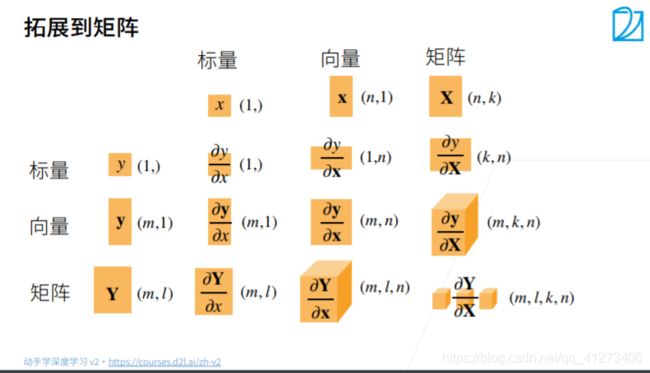
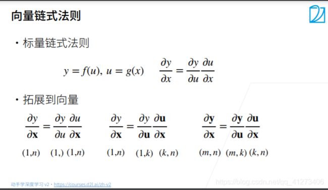
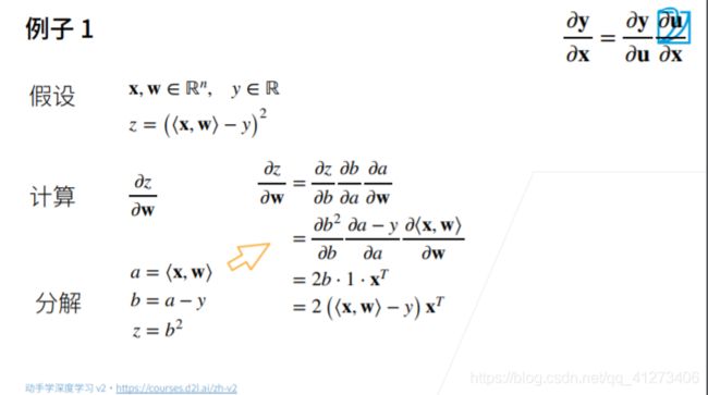
矩阵计算


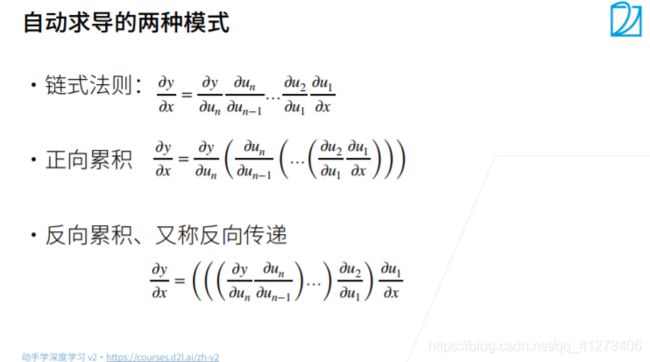
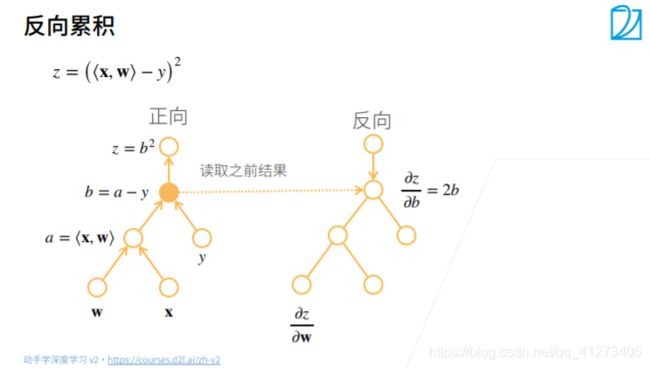
自动求导


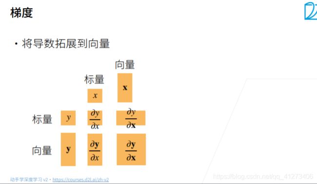
假设我们想对函数 y = 2 x ⊤ x y=2x^⊤x y=2x⊤x关于列向量 x求导
import torch

x = torch.arange(4.0)
x
tensor([0., 1., 2., 3.])
在我们计算y关于x的梯度之前,我们需要一个地方来存储梯度。
x.requires_grad_(True)  # 等价于 `x = torch.arange(4.0, requires_grad=True)`
x.grad  # 默认值是None
print(x.grad)
None
现在让我们计算 y。
y = 2 * torch.dot(x, x)
y
tensor(28., grad_fn=)
通过调用反向传播函数来自动计算y关于x 每个分量的梯度:
y.backward()
x.grad
tensor([ 0., 4., 8., 12.])
x.grad == 4 * x
tensor([True, True, True, True])
现在让我们计算 x 的另一个函数:
# 在默认情况下,PyTorch会累积梯度,我们需要清除之前的值
print(x.grad)
x.grad.zero_() #首先清零
print(x.grad)
y = x.sum()
y.backward()
x.grad
tensor([ 0.,  4.,  8., 12.])
tensor([0., 0., 0., 0.])


tensor([1., 1., 1., 1.])
深度学习中 ,我们的目的不是计算微分矩阵,而是批量中每个样本单独计算的偏导数之和:
# 对非标量调用`backward`需要传入一个`gradient`参数,该参数指定微分函数关于`self`的梯度。在我们的例子中,我们只想求偏导数的和,所以传递一个1的梯度是合适的
print(x.grad)
x.grad.zero_() #首先清零
print(x.grad)

y = x * x
# 等价于y.backward(torch.ones(len(x)))
y.sum().backward()
x.grad
tensor([1., 1., 1., 1.])
tensor([0., 0., 0., 0.])


tensor([0., 2., 4., 6.])
将某些计算移动到记录的计算图之外:
x.grad.zero_()
y = x * x
u = y.detach()
z = u * x

z.sum().backward()
x.grad == u
tensor([True, True, True, True])
x.grad.zero_()
y.sum().backward()
x.grad == 2 * x
tensor([True, True, True, True])
即使构建函数的计算图需要通过 Python控制流(例如,条件、循环或任意函数调用),我们仍然可以计算得到的变量的梯度
def f(a):
    b = a * 2
    while b.norm() < 1000:
        b = b * 2
    if b.sum() > 0:
        c = b
    else:
        c = 100 * b
    return c

a = torch.randn(size=(), requires_grad=True)
d = f(a)
d.backward()

a.grad == d / a
tensor(True)
3.27课程
线性回归


基础优化方法


线性回归从零开始实现
我们将从零开始实现整个方法,包括数据流水线,模型,损失函数和小批量随机梯度下降优化器
%matplotlib inline
import random
import torch
from d2l import torch as d2l
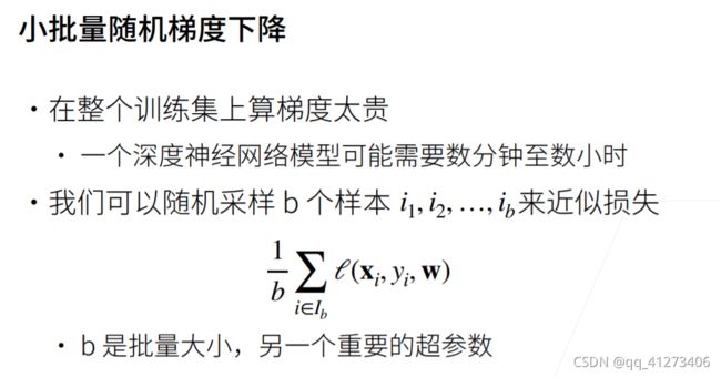
根据带有噪音的线性模型构造一个人造数据集。
使用线性模型参数 w = [ 2 , − 3.4 ] T , b = 4.2 w = [2, -3.4]^T , b = 4.2 w=[2,−3.4]T,b=4.2 和噪声项 ϵ \epsilon ϵ 生成数据集及其标签:
y = X w + b + ϵ y = Xw + b + \epsilon y=Xw+b+ϵ
def synthetic_data(w, b, num_examples):
    '''生成 y= Xw + b + 噪音'''
    X = torch.normal(0, 1, (num_examples, len(w)))
    y = torch.matmul(X, w) + b
    y += torch.normal(0, 0.01, y.shape)
    return X, y.reshape((-1, 1))

true_w = torch.tensor([2, -3.4])
true_b = 4.2
features, labels = synthetic_data(true_w, true_b, 1000)
print('features:', features[0], '\nlabel:', labels[0])
features: tensor([1.5007, 1.6155])
label: tensor([1.7014])
features.shape
torch.Size([1000, 2])
len(true_w)
2
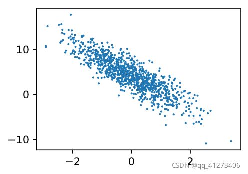
d2l.set_figsize()
d2l.plt.scatter(features[:, 1].detach().numpy(),
               labels.detach().numpy(), 1)
定义一个data_iter 函数, 该函数接受批量大小。特征矩阵和标签向量作为输入,生成大小batch_size的小批量
def data_iter(batch_size, features, labels):
    num_examples = len(features)
    indices = list(range(num_examples))# 生成下标
    # 这些样本是随机读取的,没有特定的顺序
    random.shuffle(indices)
    for i in range(0, num_examples, batch_size):#每次取batch_size个
        batch_indices = torch.tensor(indices[i:min(i + batch_size , num_examples)])
        yield features[batch_indices], labels[batch_indices] # yield 类似 return


batch_size = 10
for X, y in data_iter(batch_size, features, labels):
    print(X, '\n', y)
    break
tensor([[-0.0686,  1.6402],
        [ 0.9647, -0.6753],
        [-0.8480,  0.3525],
        [ 0.5542, -0.7129],
        [ 1.6553,  1.4655],
        [-1.0177, -0.7615],
        [ 0.6186,  2.3542],
        [-0.3753, -0.9401],
        [ 1.2845,  0.2303],
        [-0.7976,  1.7579]])
 tensor([[-1.5123],
        [ 8.4337],
        [ 1.3023],
        [ 7.7215],
        [ 2.5304],
        [ 4.7537],
        [-2.5618],
        [ 6.6497],
        [ 5.9861],
        [-3.3762]])
定义初始化模型
w = torch.normal(0, 0.01, size=(2, 1), requires_grad=True)#w 初始换为均值为0,方差为0.01的正态分布
b = torch.zeros(1, requires_grad=True)
w.shape,w
(torch.Size([2, 1]),
 tensor([[-0.0045],
         [-0.0179]], requires_grad=True))
定义模型
def linreg(X, w, b):
    """线性回归"""
    return torch.matmul(X, w)+b
定义损失函数
def squared_loss(y_hat, y):
    """均方损失"""
    return (y_hat - y.reshape(y_hat.shape))**2 / 2 / batch_size
定义优化算法
def sgd(params, lr, batch_size):
    """小批量随机梯度下降"""
    with torch.no_grad(): #更新是不需要计算梯度
        for param in params:
            param -= lr * param.grad
            param.grad.zero_()
训练过程
lr = 0.03 #学习率
num_epochs = 3 # 全程扫三遍数据
net = linreg #训练模型
loss = squared_loss

for epoch in range(num_epochs):
    for X, y in data_iter(batch_size, features, labels):
        l = loss(net(X, w, b), y)

        l.sum().backward()
        sgd([w, b], lr, batch_size) #使用参数的梯度更新参数

    with torch.no_grad():
        train_l = loss(net(features, w, b), labels)
        print(f'epoch {
       epoch + 1}, loss {
       float(train_l.mean()):f}')
epoch 1, loss 0.003963
epoch 2, loss 0.000014
epoch 3, loss 0.000005
因为数据是我们自己合成的所以可以看一下训练出的参数与真实的参数对比
print(f'w的估计误差:{
       true_w - w.reshape(true_w.shape)}')
print(f'b的估计误差:{
       true_b - b}')
w的估计误差:tensor([ 0.0004, -0.0006], grad_fn=)
b的估计误差:tensor([0.0002], grad_fn=)
print(f'w的估计误差:{
       true_w - w.reshape(true_w.shape)}')
print(f'b的估计误差:{
       true_b - b}')
w的估计误差:tensor([ 0.0004, -0.0006], grad_fn=)
b的估计误差:tensor([0.0002], grad_fn=)
线性回归的简洁实现
通过使用深度学习框架来简洁的实现线性回归模型 生成数据集
import numpy as np
import torch
from torch.utils import data
from d2l import torch as d2l

true_w = torch.tensor([2, -3.4])
true_b = 4.2
features, labels = d2l.synthetic_data(true_w, true_b, 1000)
labels.shape
torch.Size([1000, 1])
调用框架中现有的API来读取数据
def load_array(data_arrays, batch_size, is_train=True):
    """构造一个PyTorch数据迭代器"""
    dataset = data.TensorDataset(*data_arrays) # TensorDataset 将输入的两类数据一一对应
    return data.DataLoader(dataset, batch_size, shuffle=is_train)# DataLoader 重新排序

batch_size = 10
data_iter = load_array((features, labels), batch_size)

next(iter(data_iter))
[tensor([[ 2.0952, -0.6280],
         [ 0.5289, -0.6611],
         [-1.5620, -1.3813],
         [-0.9851,  2.0845],
         [ 0.1278,  1.8460],
         [-1.1976,  0.5956],
         [-0.0973,  1.2284],
         [-1.1078,  0.9514],
         [-1.6016, -1.1474],
         [ 0.8461,  0.9182]]),
 tensor([[10.5349],
         [ 7.5078],
         [ 5.7682],
         [-4.8577],
         [-1.8178],
         [-0.2159],
         [-0.1622],
         [-1.2476],
         [ 4.8937],
         [ 2.7743]])]
使用框架的预定义好的层
# nn 是神经网络的缩写
from torch import nn

net = nn.Sequential(nn.Linear(2, 1))#线性层 输入2 输出1
初始化模型参数
net[0].weight.data.normal_(0, 0.01)
net[0].bias.data.fill_(0)
tensor([0.])
计算均方误差使用的是 MSELoss 类,也称为平方 L 2 L_2 L2范数
loss = nn.MSELoss()
实例化 SGD 实例
trainer = torch.optim.SGD(net.parameters(), lr=0.03)
训练过程
num_epochs = 3
for epoch in range(num_epochs):
    for X,y in data_iter: #取出小批量
        l = loss(net(X), y)
        trainer.zero_grad()
        l.backward()
        trainer.step()
    l = loss(net(features), labels)
    print(f'epoch:{
       epoch+1}, loss:{
       l:f}')
epoch:1, loss:0.000261
epoch:2, loss:0.000093
epoch:3, loss:0.000093
比较生成数据集的真实参数和通过有限数据训练获得的模型参数
w = net[0].weight.data
print('w的估计误差:', true_w - w.reshape(true_w.shape))
b = net[0].bias.data
print('b的估计误差:', true_b - b)
w的估计误差: tensor([2.9922e-05, 4.2915e-05])
b的估计误差: tensor([-0.0005])
3.28课程
softmax回归


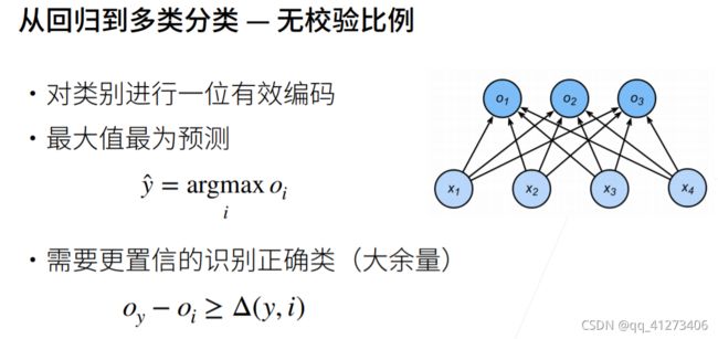

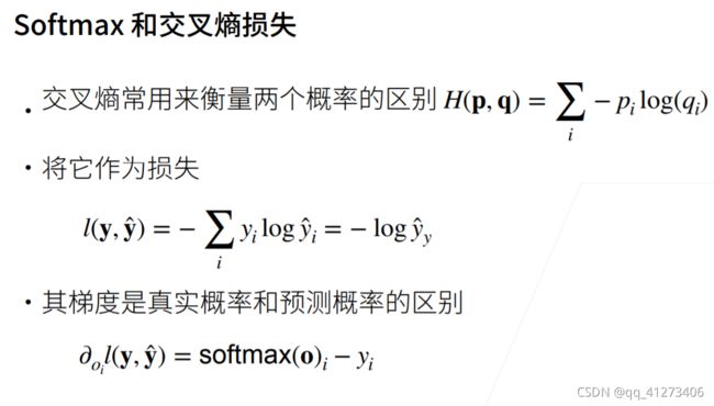

损失函数
均方损失函数
蓝色:y=0时,y’的图像
绿色:似然函数
橙色:函数的梯度(导数)

绝对值损失函数
蓝色:y=0时,y’的图像
绿色:似然函数
橙色:函数的梯度(导数)

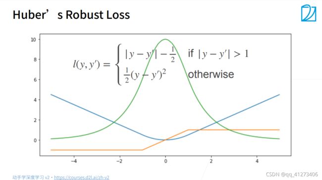
混合损失函数
蓝色:y=0时,y’的图像
绿色:似然函数
橙色:函数的梯度(导数)
优点:在比较大的地方(>1)梯度会是一个定值,当<1时梯度会逐渐减少,不会出现梯度太大找不到合适的点。
图像分类数据集
MNIST数据集是图像分类中广泛使用的数据集之一,但作为基准数据集过于简单。我们将使用类似但更复杂的Fashion-MNIST数据集
%matplotlib inline
import torch
import torchvision
from torch.utils import data
from torchvision import transforms
from d2l import torch as d2l

d2l.use_svg_display()#使用svg来显示图片
通过框架中的内置函数将 Fashion-MNIST 数据集下载并读取到内存中
# 通过ToTensor实例将图像数据从PIL类转变成32位浮点格式
# 并除以255使得所有的像素的数值在0到1之间
trans = transforms.ToTensor()
mnist_train = torchvision.datasets.FashionMNIST(root="../data", train=True, transform=trans, download=True)
mnist_test = torchvision.datasets.FashionMNIST(root="../data", train=False, transform=trans, download=True)

len(mnist_train), len(mnist_test)
D:\Anaconda3\envs\pytorch\lib\site-packages\torchvision\datasets\mnist.py:498: UserWarning: The given NumPy array is not writeable, and PyTorch does not support non-writeable tensors. This means you can write to the underlying (supposedly non-writeable) NumPy array using the tensor. You may want to copy the array to protect its data or make it writeable before converting it to a tensor. This type of warning will be suppressed for the rest of this program. (Triggered internally at  ..\torch\csrc\utils\tensor_numpy.cpp:180.)
  return torch.from_numpy(parsed.astype(m[2], copy=False)).view(*s)


(60000, 10000)
mnist_train[0][0].shape #图片 1 黑白, 长 28, 宽28
torch.Size([1, 28, 28])
mnist_train[0][1] #label
9
两个可视化数据集的函数
def get_fashion_mnist_labels(labels):
    """返回Fashion-MNIST数据集的文本标签"""
    text_labels = [
        't-shirt', 'trouser', 'pullover', 'dress', 'coat', 'sandal', 'shirt',
        'sneaker', 'bag', 'ankle boot'
    ]
    return [text_labels[int(i)] for i in labels]

def show_images(imgs, num_rows, num_cols, titles=None, scale=1.5):
    """展示图片"""
    figsize = (num_cols * scale, num_rows * scale)
    _, axes = d2l.plt.subplots(num_rows, num_cols, figsize=figsize)# _ 可以存储无用的数据
    axes = axes.flatten()
    for i, (ax, img) in enumerate(zip(axes, imgs)):
        if torch.is_tensor(img):
            ax.imshow(img.numpy())
        else:
            ax,imshow(img)
        ax.axes.get_xaxis().set_visible(False)
        ax.axes.get_yaxis().set_visible(False)
        if titles:
            ax.set_title(titles[i])
    return axes
get_fashion_mnist_labels([3,0])
['dress', 't-shirt']
几个样本的图像及其相应的标签
X, y = next(iter(data.DataLoader(mnist_train, batch_size=18)))
show_images(X.reshape(18, 28, 28), 3, 6, titles=get_fashion_mnist_labels(y))# 3行6列
array([,
       ,
       ,
       ,
       ,
       ,
       ,
       ,
       ,
       ,
       ,
       ,
       ,
       ,
       ,
       ,
       ,
       ], dtype=object)

读取一小批量数据,大小为batch_size
batch_size = 256

def get_dataloader_workers():
    """使用0个进程来读取数据。"""
    return 0 # CPU 太low

train_iter = data.DataLoader(mnist_train, batch_size, shuffle=True, # shuffle 是否随机
                             num_workers=get_dataloader_workers())

timer = d2l.Timer() # 测试速度
for X, y in train_iter:
    continue
f'{
       timer.stop():.2f} sec'
'3.92 sec'
定义 load_data_fashion_mnist 函数,以后重用
def load_data_fashion_mnist(batch_size, resize=None):
    """下载Fashion-MNIST数据集,然后将其加载到内存中"""
    trans = [transforms.ToTensor()]
    if resize: #如果图片数据不只3维,则通过resize来增加数据。
        trans.insert(0, transforms.Resize(resize))
    trans = transforms.Compose(trans)
    mnist_train = torchvision.datasets.FashionMNIST(root="../data",
                                                   train=True,
                                                    transform=trans,
                                                   download=True)
    mnist_test = torchvision.datasets.FashionMNIST(root="../data",
                                                  train=False,
                                                  transform=trans,
                                                  download=True)

    return (data.DataLoader(mnist_train, batch_size, shuffle=True,
                           num_workers=get_dataloader_workers()),
           data.DataLoader(mnist_test, batch_size, shuffle=False,
                          num_workers=get_dataloader_workers()))

train_iter, test_iter = load_data_fashion_mnist(32, resize=64)
for X, y in train_iter:
    print(X.shape, X.dtype, y.shape, y.dtype)
    break
torch.Size([32, 1, 64, 64]) torch.float32 torch.Size([32]) torch.int64
shion_mnist(32, resize=64)
for X, y in train_iter:
    print(X.shape, X.dtype, y.shape, y.dtype)
    break
torch.Size([32, 1, 64, 64]) torch.float32 torch.Size([32]) torch.int64
softmax 回归的从零开始实现
import torch
from IPython import display
from d2l import torch as d2l

batch_size = 256
train_iter, test_iter = d2l.load_data_fashion_mnist(batch_size) # 每次读取256张图片
D:\Anaconda3\envs\pytorch\lib\site-packages\torchvision\datasets\mnist.py:498: UserWarning: The given NumPy array is not writeable, and PyTorch does not support non-writeable tensors. This means you can write to the underlying (supposedly non-writeable) NumPy array using the tensor. You may want to copy the array to protect its data or make it writeable before converting it to a tensor. This type of warning will be suppressed for the rest of this program. (Triggered internally at  ..\torch\csrc\utils\tensor_numpy.cpp:180.)
  return torch.from_numpy(parsed.astype(m[2], copy=False)).view(*s)
将展平每个图像,把它们看作长度为784的向量。 因为我们的数据集有10个类别,所以网络输出维度为 10
num_inputs = 784 #28*28
num_outputs = 10 # 10类

W = torch.normal(0, 0.01, size=(num_inputs, num_outputs), requires_grad=True)
b = torch.zeros(num_outputs, requires_grad=True)
给定一个矩阵X,我们可以对所有元素求和
X = torch.tensor([[1.0, 2.0, 3.0], [4.0, 5.0, 6.0]])
X,X.sum(0, keepdim=True), X.sum(1, keepdim=True)
(tensor([[1., 2., 3.],
         [4., 5., 6.]]),
 tensor([[5., 7., 9.]]),
 tensor([[ 6.],
         [15.]]))
实现softmax
s o f t m a x ( X ) i j = e x p ( X i j ) ∑ k e x p ( X i k ) softmax(X)_{ij} = \frac{exp(X_{ij})}{\sum_k exp(X_{ik})} softmax(X)ij=∑kexp(Xik)exp(Xij)
def softmax(X):
    X_exp = torch.exp(X)
    partition = X_exp.sum(1, keepdim=True)
    return X_exp / partition # 这里应用了广播机制
我们将每个元素变成一个非负数。此外依据概率原理,每行总和为1
X = torch.normal(0, 1, (2, 5))
X_prob = softmax(X)
X_prob, X_prob.sum(1)
(tensor([[0.4321, 0.2430, 0.0155, 0.2598, 0.0496],
         [0.2585, 0.0585, 0.5983, 0.0402, 0.0446]]),
 tensor([1., 1.]))
实现softmax回归模型
def net(X):
    return softmax(torch.matmul(X.reshape((-1, W.shape[0])), W) + b)
创建一个数据y_hat,其中包含2个样本在3个类别的预测概率, 使用y作为y_hat中概率的索引
y = torch.tensor([0, 2])
y_hat = torch.tensor([[0.1, 0.3, 0.6], [0.3, 0.2, 0.5]])
y_hat[[0, 1], y], y
(tensor([0.1000, 0.5000]), tensor([0, 2]))
实现交叉熵损失函数
def cross_entropy(y_hat, y):
    return -torch.log(y_hat[range(len(y_hat)), y])

cross_entropy(y_hat, y)
tensor([2.3026, 0.6931])
将预测类别与真实 y 元素进行比较
def accuracy(y_hat, y):
    """计算预测正常的计算数量"""
    if len(y_hat.shape) > 1 and y_hat.shape[1] > 1:
        y_hat = y_hat.argmax(axis=1) # 多行中 将最大值的下标传回 y_hat中

    cmp = y_hat.type(y.dtype) == y #与真实值y比较 预测正确为1,错误为0 存在cmp中
    return float(cmp.type(y.dtype).sum())

accuracy(y_hat, y) / len(y)
0.5
评估在任意模型 net 的准确率:
def evaluate_accuracy(net, data_iter):
    """计算在指定数据集上模型"""
    if isinstance(net, torch.nn.Module):
        net.eval() # 将模型设置为评估模式
    metric = Accumulator(2) # [正确预测数, 预测总数]

    for X, y in data_iter:
        metric.add(accuracy(net(X), y), y.numel())

    return metric[0]/metric[1]
Accumulator 实例中创建了 2 个变量,用于分别存储正确预测的数量和预测的总数量
class Accumulator:
    """在`n`个变量上累加。"""
    def __init__(self, n):
        self.data = [0.0] * n

    def add(self, *args):
        self.data = [a + float(b) for a, b in zip(self.data, args)]

    def reset(self):
        self.data = [0.0] * len(self.data)

    def __getitem__(self, idx):
        return self.data[idx]
# 计算随机出来的数的精确率(10类别大约0.1的精确率)
evaluate_accuracy(net, test_iter)
0.0772
Softmax回归的训练
def train_epoch_ch3(net, train_iter, loss, updater):
    """训练模型一个迭代周期(定义见第3章)。"""
    if isinstance(net, torch.nn.Module):# 将模型设置为训练模式
        net.train()
    metric = Accumulator(3) # 训练损失总和、训练准确度总和、样本数
    for X, y in train_iter:
        y_hat = net(X)
        l = loss(y_hat, y)
        if isinstance(updater, torch.optim.Optimizer):# 使用PyTorch内置的优化器和损失函数
            updater.zero_grad()
            l.backward()
            updater.step()
            metric.add(
                float(l) * len(y), accuracy(y_hat, y),
                y.size().numel())
        else: # 自己实现
            l.sum().backward()
            updater(X.shape[0])
            metric.add(float(l.sum()), accuracy(y_hat, y), y.numel())
    return metric[0] / metric[2], metric[1] / metric[2]
在展示训练函数的实现之前,我们定义一个在动画中绘制数据的实用程序类。它能够简化本书其余部分的代码。
class Animator:  #@save
    """在动画中绘制数据。"""
    def __init__(self, xlabel=None, ylabel=None, legend=None, xlim=None,
                 ylim=None, xscale='linear', yscale='linear',
                 fmts=('-', 'm--', 'g-.', 'r:'), nrows=1, ncols=1,
                 figsize=(3.5, 2.5)):
        # 增量地绘制多条线
        if legend is None:
            legend = []
        d2l.use_svg_display()
        self.fig, self.axes = d2l.plt.subplots(nrows, ncols, figsize=figsize)
        if nrows * ncols == 1:
            self.axes = [self.axes, ]
        # 使用lambda函数捕获参数
        self.config_axes = lambda: d2l.set_axes(
            self.axes[0], xlabel, ylabel, xlim, ylim, xscale, yscale, legend)
        self.X, self.Y, self.fmts = None, None, fmts

    def add(self, x, y):
        # 向图表中添加多个数据点
        if not hasattr(y, "__len__"):
            y = [y]
        n = len(y)
        if not hasattr(x, "__len__"):
            x = [x] * n
        if not self.X:
            self.X = [[] for _ in range(n)]
        if not self.Y:
            self.Y = [[] for _ in range(n)]
        for i, (a, b) in enumerate(zip(x, y)):
            if a is not None and b is not None:
                self.X[i].append(a)
                self.Y[i].append(b)
        self.axes[0].cla()
        for x, y, fmt in zip(self.X, self.Y, self.fmts):
            self.axes[0].plot(x, y, fmt)
        self.config_axes()
        display.display(self.fig)
        display.clear_output(wait=True)
训练函数
接下来我们实现一个训练函数,它会在train_iter访问到的训练数据集上训练一个模型net。该训练函数将会运行多个迭代周期(由num_epochs指定)。在每个迭代周期结束时,利用test_iter访问到的测试数据集对模型进行评估。我们将利用Animator类来可视化训练进度。
def train_ch3(net, train_iter, test_iter, loss, num_epochs, updater):
    """训练模型(定义见第3章)。"""
    animator = Animator(xlabel='epoch', xlim=[1, num_epochs], ylim=[0.3, 0.9],
                        legend=['train loss', 'train acc', 'test acc'])
    for epoch in range(num_epochs):
        train_metrics = train_epoch_ch3(net, train_iter, loss, updater)
        test_acc = evaluate_accuracy(net, test_iter)
        animator.add(epoch + 1, train_metrics + (test_acc,))
    train_loss, train_acc = train_metrics
    assert train_loss < 0.5, train_loss
    assert train_acc <= 1 and train_acc > 0.7, train_acc
    assert test_acc <= 1 and test_acc > 0.7, test_acc
我们使用 小批量随机梯度下降来优化模型的损失函数,设置学习率为0.1
lr = 0.1

def updater(batch_size):
    return d2l.sgd([W, b], lr, batch_size)
现在,我们训练模型10个迭代周期。请注意,迭代周期(num_epochs)和学习率(lr)都是可调节的超参数。通过更改它们的值,我们可以提高模型的分类准确率。
num_epochs = 10
train_ch3(net, train_iter, test_iter, cross_entropy, num_epochs, updater)

现在训练已经完成,我们的模型已经准备好对图像进行分类预测。给定一系列图像,我们将比较它们的实际标签(文本输出的第一行)和模型预测(文本输出的第二行)。
def predict_ch3(net, test_iter, n=6):  #@save
    """预测标签(定义见第3章)。"""
    for X, y in test_iter:
        break
    trues = d2l.get_fashion_mnist_labels(y)
    preds = d2l.get_fashion_mnist_labels(net(X).argmax(axis=1))
    titles = [true +'\n' + pred for true, pred in zip(trues, preds)]
    d2l.show_images(
        X[0:n].reshape((n, 28, 28)), 1, n, titles=titles[0:n])

predict_ch3(net, test_iter)

softmax回归的简洁实现
我们可以发现通过深度学习框架的高级API能够使实现
线性回归变得更加容易。同样地,通过深度学习框架的高级API也能更方便地实现分类模型。让我们继续使用Fashion-MNIST数据集,并保持批量大小为256,
import torch
from torch import nn
from d2l import torch as d2l


batch_size = 256
train_iter, test_iter = d2l.load_data_fashion_mnist(batch_size)
D:\Anaconda3\envs\pytorch\lib\site-packages\torchvision\datasets\mnist.py:498: UserWarning: The given NumPy array is not writeable, and PyTorch does not support non-writeable tensors. This means you can write to the underlying (supposedly non-writeable) NumPy array using the tensor. You may want to copy the array to protect its data or make it writeable before converting it to a tensor. This type of warning will be suppressed for the rest of this program. (Triggered internally at  ..\torch\csrc\utils\tensor_numpy.cpp:180.)
  return torch.from_numpy(parsed.astype(m[2], copy=False)).view(*s)
初始化模型参数
softmax回归的输出层是一个全连接层。因此,为了实现我们的模型,我们只需在Sequential中添加一个带有10个输出的全连接层。同样,在这里,Sequential并不是必要的,但我们可能会形成这种习惯。因为在实现深度模型时,Sequential将无处不在。我们仍然以均值0和标准差0.01随机初始化权重。
# PyTorch不会隐式地调整输入的形状。因此,
# 我们在线性层前定义了展平层(flatten),来调整网络输入的形状
net = nn.Sequential(nn.Flatten(), nn.Linear(784, 10))

def init_weights(m):
    if type(m) == nn.Linear:
        nn.init.normal_(m.weight, std=0.01)

net.apply(init_weights);
在交叉熵损失函数中传递未归一化的预测,并同时计算softmax及其对数
loss = nn.CrossEntropyLoss()
使用学习率为0.1的小批量随机梯度下降作为优化算法
trainer = torch.optim.SGD(net.parameters(), lr=0.1)
调用 之前 定义的训练函数来训练模型
num_epochs = 10
d2l.train_ch3(net, train_iter, test_iter, loss, num_epochs, trainer)
