机器学习-梯度下降-2020-3-2
What is Gradient Descent?(慢慢看,英语有点吃力,不过质量还不错)
https://www.analyticsvidhya.com/blog/2017/03/introduction-to-gradient-descent-algorithm-along-its-variants/
-----------------------------------------------------------------------------
基本概率:
-----------------------------------------------------------------------------
什么是梯度?
就是函数变化增加最快的地方,一元函数,就是导数的概念。
梯度下降(gradient descent)法用来做什么?
求无约束的函数的极小值。(注意全局极小值 global minimum,局部极小值 local minima)
对有约束问题的:一般用拉格朗日乘数法,考研经常做
应用:
线性回归,Logistic 回归等,通过迭代,找出目标函数的最小值。
凸函数的数学定义:
某个向量空间的凸子集(区间)上的实值函数,如果在其定义域上的任意两点,有 f(tx1+ (1-t)x2) <= tf(x1) + (1-t)f(x2),则称其为该区间上的凸函数。
使用梯度下降注意条件:
在应用任何算法之前,先确定它是凸函数。
1:当目标函数是凸函数时,梯度下降法的解是全局解( global minimum)。(数学证明,凸优化理论)一般情况下,其解不保证是全局最优解,梯度下降法的速度也未必是最快的。
2:翻译不好,就不翻译了。
There is also a saddle point problem. (鞍点问题)This is a point in the data where the gradient is zero but is not an optimal point. We don’t have a specific way to avoid this point and is still an active area of research.
3:算法参数初始化的选择。 一般用随机数生成
4:数据的归一化处理
缺点
-
1:由于许多问题是非强凸或良态的,因此梯度下降往往需要很多次迭代,收敛速度很慢;
-
2:不能应对不可微的函数。
-
3: 靠近极小值时收敛速度减,开始快,后面越来越慢越接近目标值,步长越小,前进越慢
-
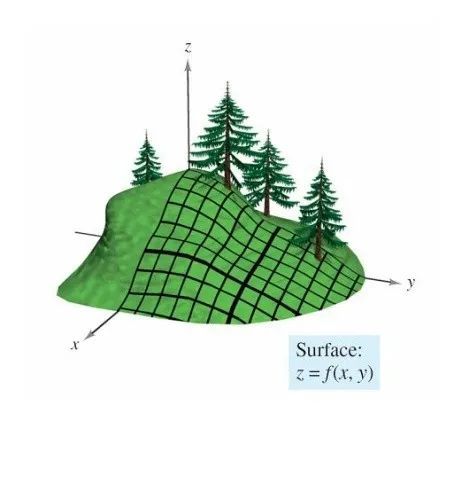
假设这样一个场景:(形象理解)
一个人在山上,怎么最快速下山?
首先是面临两个选择: 决定走的方向(四面八方,朝哪个方向go),和步长(一步子走多少)
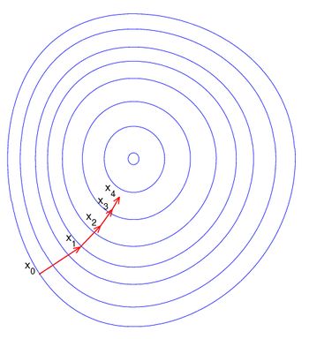
理想情况:以他当前的所处的位置为基准,寻找这个位置最陡峭的地方,然后朝着下降方向走一步,然后又继续以当前位置为基准,再找最陡峭的地方,再走直到最后到达最低处。

在多变量函数中,梯度是一个向量,向量有方向,梯度的方向就指出了函数在给定点的上升最快的方向,加个负号,就是下降得最快的方向。
梯度:grad(f(x, y) ) = ▽ f(x,y)


Learning_rate : 学习步长 (适当 0.01 , 0.05 之间过大过小都不好
步长太大,会导致迭代过快,甚至有可能错过最优解。
步长太小,迭代速度太慢,很长时间算法都不能结束。
hypothesis function : 假设函数 , 也是模型函数
Loss function :损失函数 , 也就是我们要优化的函数。
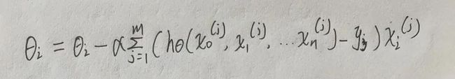
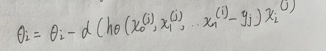
梯度下降法的代数方式描述:
------------------------------------------------------------------------------
eg: 简单 一元线性回归实例
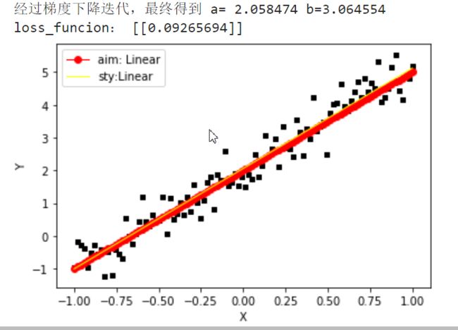
利用上面推导的公式实现: y = 3*x + 2
人工制造数据集:
随机生成一个近似采样随机分布,使得θ0=2.0, θ1=3, 并加入一个噪声,噪声的最大振幅为0.4
------------------------------------------------------------------------------
import numpy as npimport matplotlib.pyplot as pltdef loss_Function(theta,x,y,m):"""theta: [ [θ1],[θ2] ] 待求参数 shape : 2*1x : 数据集 m *[x0,x1] shape: m *2y : 标签值 shape: m *1m : 数据集个数"""# 均方差Subtraction =np.dot(x,theta) -ysquare = 1/(2*m)*np.dot(np.transpose(Subtraction) ,Subtraction)return square#定义代价函数对应的梯度函数def gradinet_Function(theta,x,y,m):"""theta: [ [θ1],[θ2] ] 待求参数 shape :2*1x : 数据集 m *[x0,x1] shape: m *2y : 标签值 shape: m *1m : 数据集个数"""#参照矩阵求导公式diff = np.dot(x,theta)-ysquare =1/m*np.dot(np.transpose(x),diff)return squaredef gradient_Descent():theta = np.array([1, 1]).reshape(2, 1) # 初始化theta ,默认为 1gradient = gradinet_Function(theta,x,y,data_num) #计算梯度while not all(np.abs(gradient) <= 1e-5): # 迭代结束条件,1e-5 ,可以认为无穷小量theta = theta -learning_rate*gradient #更新thetagradient = gradinet_Function(theta,x,y,data_num)# 求当前位置梯度return thetadef plot_(theta,x,y):ax = plt.subplot(111)ax.scatter(x, y, s=10, marker="s",color='black')plt.xlabel("X")plt.ylabel("Y")#目标直线plt.plot(x_data,3*x_data+2.0, linewidth = '1',color='red',label='aim: Linear',marker='o')#学习直线y1 = theta[0] + theta[1]*xax.plot(x, y1,linewidth = '1',color='yellow',label="sty:Linear")plt.legend(loc='upper left')plt.show()learning_rate = 0.01# np.linspace 生成等差数列在-(-1,1)之间 100个点x_data = np.linspace(-1,1,100)# *x_data.shape 将转成数字 标准正态分布。y_data = 3*x_data +2.0+np.random.randn(*x_data.shape)*0.4#plt.plot(x_data, y_data, 'go', label='Original data') #画出数据集的图像data_num = x_data.shape[0] # 获取数据集的大小x0= np.ones((data_num, 1)) #扩充矩阵 x0一列都等于1,便于矩阵运算x=x_data.reshape((data_num,1))x =np.hstack((x0,x)) #按照列堆叠形成数组,其实就是 m*[x0,x1]样本数据y=y_data.reshape((data_num,1))# 梯度下降迭代theta= gradient_Descent()print("经过梯度下降迭代,最终得到 a= %0.6f b=%0.6f"%(theta[0],theta[1]))print("loss_funcion:",loss_Function(theta,x,y,data_num))plot_(theta,x[:,1],y)
结果非常接近我们预期的估计值了!
批量梯度下降法(Batch Gradient Descent)
在更新参数时使用所有的样本来进行更新:
随机梯度下降法(Stochastic Gradient Descent)
与批量梯度 下降相反:仅仅是随机选取一个样本j 来求梯度,进行更新
小批量梯度下降法(Mini-batch Gradient Descent)
小批量梯度下降法是批量梯度下降法和随机梯度下降法的折衷,也就是对于m个样本,我们采用x个样本来迭代,1 ------------------------------------------------------------------------------ eg: 利用梯度下降求 fxy = (x-10)^2 + (y-10)^ 的最小值 容易看出最小值:当 x = 10 , y= 10 ,fxy取最小值 =0 ------------------------------------------------------------------------------ 代码实现: 看结果:x,y 非常接近我们预想的x,y=10, 最小值可以近似看成0 这些小点连成的直线就是: 我们最快下山的路线。 这是fxy值得变化图像,可值fxy最后在0处收敛 参考: https://www.cnblogs.com/pinard/p/5970503.html#!comments http://papers.nips.cc/paper/3793-efficient-learning-using-forward-backward-splitting.pdf https://www.analyticsvidhya.com/blog/2017/03/introduction-to-gradient-descent-algorithm-along-its-variants/ 
"""eg: 利用梯度下降求 fxy = (x-10)^2 + (y-10)^ 的最小值 容易看出最小值:当 x = 10 , y= 10 ,fxy =0"""import matplotlib.pyplot as plt import numpy as np from mpl_toolkits.mplot3d import Axes3D#lossfunctiondef function_xy(x,y): """ x: 自变量 y: 自变量 return : 返回函数运算结果 """ return (x-10)**2 +(y-10)**2#梯度下降def gradient_descent(): learing_rate = 0.02 #学习率,步长 x=tf.constant(20.0) #初始值 y=tf.constant(20.0) #画出3维立体图 fig = Axes3D(plt.figure()) #将figure转化为3D xp = np.linspace(0,20,100) yp = np.linspace(0,20,100) xp,yp = np.meshgrid(xp,yp) #将数据转化为网格数据 zp = function_xy(xp,yp) #画出x,y 范围 [0,20]的fxy图像 fig.plot_surface(xp, yp, zp, rstride=1, cstride=1, cmap=plt.get_cmap('rainbow')) while not function_xy(x,y) <=1e-5: # 迭代结束条件,1e-5 ,可以认为无穷小量 x_foot =x #画出 x,y 的下降足迹 y_foot =y f_foot =function_xy(x,y) fxy_history.append(f_foot) # 记录fxy值的变化 with tf.GradientTape(persistent=True,watch_accessed_variables=True) as tape: tape.watch([x,y]) z = function_xy(x,y) #更新参数 tape.gradient(target=z,sources=x) 是分别对x ,y 求偏导 x = x -learing_rate *tape.gradient(target=z,sources=x) y = y -learing_rate *tape.gradient(target=z,sources =y) f = function_xy(x,y) #更新后的的位置值 # x,y 足迹走向 fig.plot([x_foot, x], [y_foot, y], [f_foot, f], 'ko', lw=2, ls='-') return x,yfxy_history = [] # # 记录fxy值的变化x,y =gradient_descent() print("最后得到:当x:%f, y:%f ,fxy取得最小值:%f" % (x,y,function_xy(x,y)))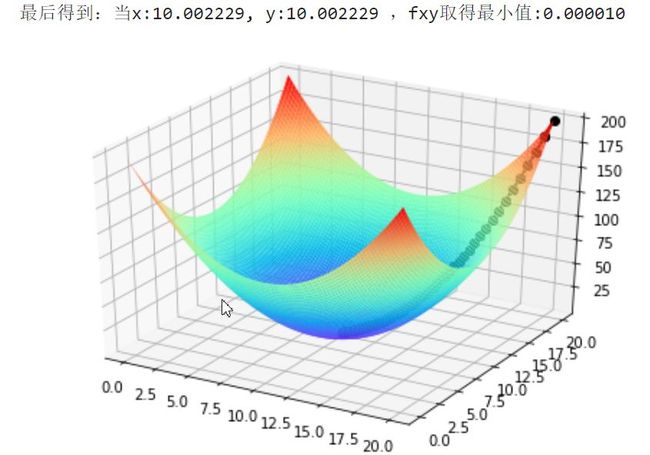
# 观察 fxy的值ax = plt.subplot(111) y =np.array(fxy_history)ax.plot(y)