10X单细胞（10X空间转录组）数据分析之cluster是否包含有意义的subcluster（SIGMA）

hello，大家好，今天我们来分享一个实用的方法，SIGMA，这个方法是用来做什么的呢？？就是说我们对一个样本进行初次聚类之后，很多时候我们需要对一个cluster再分群看看，是否一个cluster内部也具有异质性，从而挖掘有意义的新的细胞类型，那如何判断一个cluster是否值得再分群分析呢？？这个软件可以辅助我们来分析一下，文章在A clusterability measure for single-cell transcriptomics reveals phenotypic subpopulations,我们简单回顾一下文献，重点看看实例代码。

文章最重要的结论就是对每个cluster计算一个SIGMA值，值越接近于1，说明一个cluster越包含有意义的subcluster，很有必要进行cluster的再分群分析。

Abstract

The ability to discover new cell populations by unsupervised clustering of single-cell transcriptomics data has revolutionized biology（这个应该是共识了）. Currently, there is no principled way to decide, whether a cluster of cells contains meaningful subpopulations that should be further resolved（当前，没有主要的方法来确定一群细胞是否包含有意义的亚群）. Here we present SIGMA, a clusterability measure derived from random matrix theory（随机矩阵理论）, that can be used to identify cell clusters with non-random sub-structure, testably leading to the discovery of previously overlooked phenotypes.

Main，这个地方我们总结一下

1、All existing clustering algorithms have adjustable parameters, which have to be chosen carefully to reveal the true biological structure of the data

2、If the data is over-clustered, many clusters are driven purely by technical noise and do not reflect distinct biological states.（不能分群过细）。

3、If the data is under-clustered, subtly distinct phenotypes might be grouped with others and will thus be overlooked.（分群数过少容易掩盖一部分异质性）。

4、现有的评估聚类质量的工具（例如广泛使用的轮廓系数）无法揭示聚类内的可变性是否是由于亚群或随机噪声的存在。

5、为了缓解这个问题，作者开发了软件SIGMA，We consider clusterability to be the theoretically achievable agreement with the unknown ground truth clustering, for a given signal-to-noise ratio.

6、Importantly, our measure can estimate the level of achievable agreement without knowledge of the ground truth

7、High clusterability (indicated by SIGMA close to 1) means that multiple phenotypic subpopulations are present and clustering algorithms should be able to distinguish them.

8、Low clusterability (indicated by SIGMA close to 0) means that the noise is too strong for even the best possible clustering algorithm to find any clusters accurately.（内部几乎没有异质性了）。

9、If SIGMA equals 0, the observed variability within a cluster is consistent with random noise.（这个时候不需要进行再分群分析）。

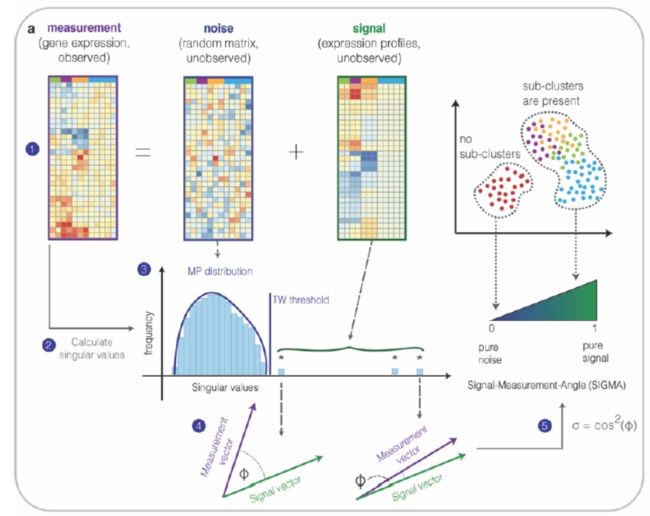
为了得出SIGMA值，我们将未观察到的实际基因表达谱（信号矩阵）视为对随机噪声矩阵的扰动 ，如下图：

图片.png

Our point of view allowed us to leverage well-established results from random matrix theory and perturbation theory。(随机矩阵理论和扰动理论)。

• first calculate the singular value(奇异值) distribution of the measured expression matrix。

if the data is preprocessed appropriately，如下图：

图片.png

the bulk of this distribution is described by the Marchenko-Pastur (MP) distribution（随机高维矩阵）, which corresponds to the random component of the measurement. The singular values outside of the MP distribution and above the Tracy Widom (TW) threshold correspond to the signal,这个地方有点难理解，因为涉及到很深的统计学知识，首先我们需要知道随机高位矩阵计算出来的奇异值符合MP分布，如果我们得到的矩阵计算出来的奇异值在这个分布以外，说明并非随机造成，而是真正的信号,不过我们简单理解一下就是高出MP分布就是我们需要的signal（当然，有一定的阈值）。接下来就是计算SIGMA值。

这个地方要注意一下：Using just these singular values and the dimensions of the measurement matrix, we can calculate the angles between the singular vectors of the measured expression matrix and those of the (unobserved) signal matrix（实际得到的矩阵和信号矩阵两个奇异值向量的角度，不知道大家还知不知道两个向量怎么求夹角，不会的翻一翻大学线性代数的书吧，作者也需要充充电了）。SIGMA is the squared cosine of the smallest angle。（SIGMA值的由来）。

Data sets with higher signal-to-noise ratios have more easily separable clusters and larger singular values outside of the MP distribution

图片.png

By definition, that results in higher values of SIGMA

图片.png

依据这个理论，我们来看看这个例子

图片.png

图上可知，再结合之前的介绍，SIGMA值越大，越包含有意义的subcluster。

图片.png

结论也是一样的。

我们重点看看示例代码

加载包

library(SIGMA)
library(ggplot2)
library(Seurat)

The authors who have anlyzed this data already normalized the data set with the R package “scran” and determined clusters by hierachical clustering. In total they have found 22 clusters.

data("force_gr_kidney")
data("sce_kidney")

paga.coord$Group <- sce_kidney$cell.type

ggplot(paga.coord, aes(x = V1, y = V2, colour = Group)) +
  geom_point(shape = 16)

图片.png

With SIGMA, we are now able to assess the variability for each cluster and see if possible sub-clusters can be found. First, we load the preprocessed SingleCellObject of the kidney data.

#Load kidney data from package

#Extract scran normalized counts and log-transform
expr.norm.log <- as.matrix(log(assay(sce_kidney, "scran")+1))

#Change the name of the rows to readable gene names
rownames(expr.norm.log) <- as.character(rowData(sce_kidney)$HUGO)
rownames(sce_kidney) <- as.character(rowData(sce_kidney)$HUGO)

In the next step we would like to exclude certain variances from appearing in the measure. For example, in this fetal kidney data set, several factors would not be of interest to cluster on: cell cycle related variances, ribosomal and mitochondrial gene expression. As, well as stress related genes, which arise during dissociation. Cycling genes, we determine here with the Seurat package, so for that we first need to create a Seurat object and normalize it. Another important factor is technical variability, for example the varying number of transcripts. It’s important to also include that in the data frame.

#Creating Seurat object
cnts <- counts(sce_kidney)
colnames(cnts) <- 1:ncol(cnts)
rownames(cnts) <- as.character(rowData(sce_kidney)$HUGO)

fetalkidney <- CreateSeuratObject(cnts)
#> Warning: Non-unique features (rownames) present in the input matrix, making unique
#> Warning: Feature names cannot have underscores ('_'), replacing with dashes ('-')
fetalkidney <- NormalizeData(fetalkidney)

#Cell cycle analysis
s.genes <- cc.genes$s.genes
g2m.genes <- cc.genes$g2m.genes

fetalkidney <- CellCycleScoring(fetalkidney, s.features = s.genes, g2m.features = g2m.genes, set.ident = TRUE)
#> Warning: The following features are not present in the object: MLF1IP, not searching for symbol synonyms

#Determining the expression of MT-genes, Rb-genes and stress genes:
data("ribosomal_genes")
data("stress_genes")

rb <- rownames(fetalkidney) %in% rb.genes 
stress.genes <- intersect(stress.genes, rownames(expr.norm.log))

#Creating the final data frame with all the factors to be excluded from considering while calculating the clusterability measure:
exclude <- data.frame(clsm = log(colSums(cnts) + 1), cellcycle = fetalkidney$G2M.Score, 
                      mt = colMeans(expr.norm.log[grep("^MT-", rownames(expr.norm.log)),]), 
                      ribosomal = colMeans(expr.norm.log[rb,]), stress = colMeans(expr.norm.log[stress.genes,]))

Now we are ready to apply the main function to determine clusterability:

out_kidney <- sigma_funct(expr.norm.log, clusters = sce_kidney$cell.type, exclude = exclude)

We can have a look at the main output of this function. For each cluster, the corresponding clusterability measure is shown.

#Evaluate the output of the measure

#plot all values for sigma
plot_sigma(out_kidney)

图片.png

值越大，越包含有意义的subcluster。

If you would like to go into more detail, then you can have a look at all sigmas and g-sigmas that are available per cluster.

#Plot all values for sigma and g_sigma
plot_all_sigmas(out_kidney)

图片.png

plot_all_g_sigmas(out_kidney)

图片.png

Data sets with higher signal-to-noise ratios are characterized by higher values of G-SIGMA。（这个地方文中提到，which indicates a more accurate estimation of differential gene expression after sub-clustering.Our approach thus not only identifies relevant sub-structure in a cell cluster but can also reveal the genes responsible for it. This is not a direct replacement for differential expression tests, but 106 a way to understand the variability within the cell-singular vectors.）

If you are interested in the values of all sigmas, g-sigmas and singular values of the signal matrix, then this information can be obtained with the help of this function.

#obtain the values for sigma and additional information
get_info(out_kidney, "UBCD")
#>        sigma   g_sigma     theta    r2vals singular_value celltype
#> 16 0.9718702 0.7595932 1.8030720 0.4468447              1     UBCD
#> 17 0.9613534 0.7073134 1.5854881 0.1810414              2     UBCD
#> 18 0.8545601 0.4459294 0.9704636 0.4134855              3     UBCD
#> 19 0.8649745 0.4617228 0.9958318 0.1402408              4     UBCD
#> 20 0.8749372 0.4779268 1.0228843 0.1069279              5     UBCD
#> 21 0.0000000 0.0000000 0.5170606 0.4340084              6     UBCD
#> 22 0.0000000 0.0000000 0.5170606 0.2978763              7     UBCD
#> 23 0.0000000 0.0000000 0.5170606 0.2157584              8     UBCD

Now, to determine if the clustrs with a high clusterability measure have variances that are meaningful for you to sub-cluster, have a look at the variance driving genes, which will tell you which genes cause the signal to appear. For example, if genes are only related to differentiation, then sub-clustering might not be necessary but could be of interest.

#See which genes cause variances in the data
get_var_genes(out_kidney, "UBCD")[,1:3]
#>            Singular.vector.1 Singular.vector.2 Singular.vector.3
#> Highest-1               RPS6              HES1               CLU
#> Highest-2              DHRS2               FOS              CTSH
#> Highest-3             SPINK1               ID2             MGST3
#> Highest-4             S100A6               ID1             EPCAM
#> Highest-5               HPGD               JUN             CYB5A
#> Highest-6              VSIG2             DDIT4             GSTM3
#> Highest-7               KRT7              JUNB               CD9
#> Highest-8              FXYD3             DUSP1             GSTP1
#> Highest-9              FBLN1           GADD45B              CD24
#> Highest-10             S100P          HSP90AB1            TUBA4A
#> Highest-11           S100A11             ADIRF              DDX5
#> Highest-12             ADIRF             RGS16              SKP1
#> Highest-13              SNCG              IER2              AGR2
#> Highest-14             PVALB             FABP5           S100A11
#> Highest-15             UPK1A               ID3              MYL6
#> Highest-16             UQCRQ             TXNIP          HSP90AB1
#> Highest-17             RPS18             H3F3A              ENO1
#> Highest-18            HMGCS2               UBB            TSPAN1
#> Highest-19              FTH1            HSPA1A             ITM2B
#> Highest-20              PSCA              RBP1            MYL12B
#> Highest-21             ADH1C              GPC3              ARG2
#> Highest-22             RPL34              IGF2             CALM2
#> Highest-23            LGALS3             SPARC              KRT8
#> Highest-24             RPL31          HSP90AA1            MYL12A
#> Highest-25           SHROOM1              TPM2             H3F3B
#> Highest-26             LEAP2              SNCG             SYPL1
#> Highest-27              UPK2           TSC22D1          LGALS3BP
#> Highest-28             CISD3            HSPA1B             KRT19
#> Highest-29             RPLP1            LGALS1             GAPDH
#> Highest-30            MT-ND3              SMC2             CLIC1
#> Highest-31             RPL12         HNRNPA2B1              RGS2
#> Highest-32              IGF2             MYLIP            MALAT1
#> Highest-33            S100A4             CALD1              CAPG
#> Highest-34              PERP             HMGB2         LINC00675
#> Highest-35            MT-ND4             NR2F1              AOC1
#> Highest-36             FABP5            YME1L1             GATA2
#> Highest-37              FBP1            COL1A2            SCPEP1
#> Highest-38             GDF15             NR2F2          TMEM176B
#> Highest-39             RPL26             SEPT7             ACTG1
#> Highest-40           MT-ATP6              IDH1             HSPA5
#> Highest-41           C9orf16           TMSB15A             DEGS2
#> Highest-42             RPS14            ZNF503               UBC
#> Highest-43             RPL41            DNAJA1             CLDN7
#> Highest-44             FAM3B             DDIT3              CAPS
#> Lowest-1              TMSB4X            PHLDA2              RPS2
#> Lowest-2             NGFRAP1              AQP2            COL1A2
#> Lowest-3                ACTB         TNFRSF12A            COL3A1
#> Lowest-4              IGFBP7             KRT18            COL1A1
#> Lowest-5               WFDC2            ERRFI1            RPL13A
#> Lowest-6               CLDN3             RPL41             RPL13
#> Lowest-7              NDUFA4              HES4               PTN
#> Lowest-8                MEST              SAT1             RPL28
#> Lowest-9               HINT1               CLU              RPS3

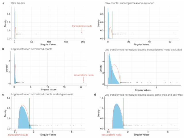
You can also check out the fit of the MP distribution for each cluster.

#Check if the MP distribution fits to the data
plot_MP(out_kidney, "UBCD")

图片.png

And for fruther validation, see if the singular vectors of the significant singular values look meaningful. By plotting either clusters or genes with the singular vectors.

#Plot clusters
plot_singular_vectors(out_kidney, "UBCD", colour = sce_kidney@metadata$ubcd.cluster)

图片.png

#Plot variance driving genes
plot_singular_vectors(out_kidney, "UBCD", colour = "UPK1A", scaled = FALSE)

图片.png

总而言之一句话，SMGMA值越接近于1，越包含有意义的subcluster，越要进行cluster的再分群分析。

生活很好，等你超越