机器学习实战—逻辑回归—信用卡欺诈检测

---

前言

最近准备开始学习机器学习，后续将对学习内容进行记录，该文主要针对通过逻辑回归模型的调优，得到较为准确可靠的反欺诈检测方法进行记录！

---

一、逻辑回归是什么？

逻辑回归概念篇可看博主之前的文章，传送门

---

二、代码实现

1.数据说明

某银行为提升信用卡反欺诈检测能力，提供了脱敏后的一份个人交易记录。考虑数据本身的隐私性，数据提供之初已经进行了类似PCA的处理，并得到了若干数据特征。
数据源下载：数据下载 提取码:vwnv

数据导入

#三大件
import numpy as np
import pandas as pd
import matplotlib.pyplot as plt
%matplotlib inline   
# 可以在Ipython编译器里直接使用，功能是可以内嵌绘图，并且可以省略掉plt.show()这一步
data = pd.read_csv("creditcard.csv")#信用卡欺诈案例，表明数据中有正常的也有不正常的，认为0正常（0多1少），1不正常，二分类问题，分类任务——逻辑回归
data.head() #v1-v28已经进行了特征的降维，直接用就可以了，但Amount需要进行预处理

输出为：

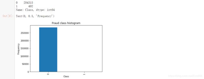
可以看到数据一共有31列，其中第一个特征Time为无用特征，V1—V28为有效特征且已经进行了特征的降维，可以直接用，Amount需要进行预处理，Class代表分类，为0表示正常，1为异常

计算正常数据与异常数据个数，并用条形图绘制

count_classes = pd.value_counts(data['Class'], sort = True)
print(count_classes)
count_classes.plot(kind = 'bar')
plt.title("Fraud class histogram")
plt.xlabel("Class")
plt.ylabel("Frequency")

输出为

2.数据预处理

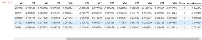
（1）无用特征删除、标准差标准化

from sklearn.preprocessing import StandardScaler #    调用sklearn的processing模块中的标准化函数，fit_transform表示对数据进行变

data['normAmount'] = StandardScaler().fit_transform(data['Amount'].values.reshape(-1, 1)) #-1让它自动去猜多少行
data = data.drop(['Time','Amount'],axis=1)#无用特征删除
data.head()

输出为：

（2）样本不平衡问题
①特征：
所谓的类别不平衡问题指的是数据集中各个类别的样本数量极不均衡。以二分类问题为例，假设正类的样本数量远大于负类的样本数量，通常情况下把样本类别比例超过4:1（也有说3:1）的数据就可以称为不平衡数据。
②影响：
简单来讲，样本不平衡会使得我们的分类模型存在很严重的偏向性，但是从一些常用的指标上又无法看出来。举一个极端一点的例子，如果正负样本比例为100:1,那岂不是把全部样本都判定为正样本就有99%+的分类准确率了。
③解决办法：
下采样：从多数集中选出一部分数据与少数集重新组合成一个新的数据集
过采样：根据样本标签少的样本的规律去生成更多该标签样本，这样使得数据趋向于平衡

3.利用下采样处理数据并进行模型训练

（1）下采样代码实现：

#先对数据进行切分
X = data.iloc[:, data.columns != 'Class']#特征数据
y = data.iloc[:, data.columns == 'Class']#label值

# Number of data points in the minority class
number_records_fraud = len(data[data.Class == 1]) #异常数据个数
fraud_indices = np.array(data[data.Class == 1].index) #异常数据的index

# Picking the indices of the normal classes
normal_indices = data[data.Class == 0].index #正常数据的index

# Out of the indices we picked, randomly select "x" number (number_records_fraud)
random_normal_indices = np.random.choice(normal_indices, number_records_fraud, replace = False)#从正常数据的index中随机选择异常数据个数的数据
random_normal_indices = np.array(random_normal_indices)#选择出来的正常数据index

# Appending the 2 indices
under_sample_indices = np.concatenate([fraud_indices,random_normal_indices])#合并在一起

# Under sample dataset
under_sample_data = data.iloc[under_sample_indices,:]#根据index获取正常、异常数据的样本

X_undersample = under_sample_data.iloc[:, under_sample_data.columns != 'Class']
y_undersample = under_sample_data.iloc[:, under_sample_data.columns == 'Class']

# Showing ratio
print("Percentage of normal transactions: ", len(under_sample_data[under_sample_data.Class == 0])/len(under_sample_data))
print("Percentage of fraud transactions: ", len(under_sample_data[under_sample_data.Class == 1])/len(under_sample_data))
print("Total number of transactions in resampled data: ", len(under_sample_data))

（2）数据集划分

from sklearn.model_selection import train_test_split

# Whole dataset
X_train, X_test, y_train, y_test = train_test_split(X,y,test_size = 0.3, random_state = 0)#random_state表示进行洗牌操作

print("Number transactions train dataset: ", len(X_train))
print("Number transactions test dataset: ", len(X_test))
print("Total number of transactions: ", len(X_train)+len(X_test))

# Undersampled dataset 用下采用数据集进行训练，但是最终需要用原数据集再进行测试，故需要对原始数据集进行切分
X_train_undersample, X_test_undersample, y_train_undersample, y_test_undersample = train_test_split(X_undersample
                                                                                                   ,y_undersample
                                                                                                   ,test_size = 0.3
                                                                                                   ,random_state = 0)
print("")
print("Number transactions train dataset: ", len(X_train_undersample))
print("Number transactions test dataset: ", len(X_test_undersample))
print("Total number of transactions: ", len(X_train_undersample)+len(X_test_undersample))

（3）交叉验证
若不采用交叉验证，直接对数据集合进行划分，如果我们的训练集和测试集的划分方法不够好，很有可能无法选择到最好的模型与参数。这里就引入了交叉验证，交叉验证，顾名思义，就是重复的使用数据，把得到的样本数据进行切分，组合为不同的训练集和测试集，用训练集来训练模型，用测试集来评估模型预测的好坏。在此基础上可以得到多组不同的训练集和测试集，某次训练集中的某样本在下次可能成为测试集中的样本，即所谓“交叉”。
那么一般在什么时候使用交叉验证呢？交叉验证用在数据不是很充足的时候。
交叉验证分为三种：
①简单交叉验证
所谓的简单，是和其他交叉验证方法相对而言的。首先，我们随机的将样本数据分为两部分（比如： 70%的训练集，30%的测试集），然后用训练集来训练模型，在测试集上验证模型及参数。接着，我们再把样本打乱，重新选择训练集和测试集，继续训练数据和检验模型。最后我们选择损失函数评估最优的模型和参数。　
②K折交叉验证（以5折交叉验证为例）

图上面的部分表示我们拥有的数据，而后我们对数据进行了再次分割，主要是对训练集，假设将训练集分成5份（该数目被称为折数，5-fold交叉验证），每次都用其中4份来训练模型，粉红色的那份用来验证4份训练出来的模型的准确率，记下准确率。然后在这5份中取另外4份做训练集，1份做验证集，再次得到一个模型的准确率。直到所有5份都做过1次验证集，也即验证集名额循环了一圈，交叉验证的过程就结束。算得这5次准确率的均值。留下准确率最高的模型，即该模型的超参数是什么样的最终模型的超参数就是这个样的。
③留一交叉验证
第三种是留一交叉验证（Leave-one-out Cross Validation），它是第二种情况的特例，此时K等于样本数N，这样对于N个样本，每次选择N-1 个样本来训练数据，留一个样本来验证模型预测的好坏。此方法主要用于样本量非常少的情况，比如对于普通适中问题， N 小于50时，我一般采用留一交叉验证。
（4）正则化惩罚项
在训练数据不够多时，或者过度训练模型时，常常会导致过拟合。正则化方法即为在此时向原始模型引入额外信息，以便防止过拟合和提高模型泛化性能的一类方法的统称，这就引入了正则化惩罚项。在实际中，最好的拟合模型（从最小化泛化误差的意义上来说）是一个适当正则化的模型。
（5）混淆矩阵

注意区分TP、TN、FP、FN，第一个字母T/F代表预测正确/错误，第二个字母P/N代表正类/负类,于是：
TP：预测正确，且判定其分类为正类 ——>正类判定为正类
FP：预测错误，且判定其分类为正类 ——>负类判定为正类
TN：预测正确，且判定其分类为负类 ——>负类判定为负类
FN：预测错误，且判定其分类为负类 ——>正类判定为负类
 
模型评估相关指标
准确率：预测正确的样本数(TP和TN)占所有样本数的比例，一般地说，准确率越高，分类器越好，计算公式如下：
$$Acc=\frac{TP+TN}{TP+TN+FP+FN}$$
精确率：正确预测为正的样本数(TP)占全部预测为正(TP和FP)的比例，计算公式如下：
$$Precision=\frac{TP}{TP+FP}$$
召回率：正确预测为正的样本数(TP)占全部实际为正(TP和FN)的比例，计算公式如下：
$$Recall=\frac{TP}{TP+FN}$$
（6）通过交叉验证找最佳惩罚力度代码

def printing_Kfold_scores(x_train_data,y_train_data):
    fold = KFold(5,shuffle=False)   #切分成五部分
    # Different C parameters 正则化惩罚项
    c_param_range = [0.01,0.1,1,10,100]#设置惩罚力度

    results_table = pd.DataFrame(index = range(len(c_param_range),2), columns = ['C_parameter','Mean recall score'])
    results_table['C_parameter'] = c_param_range

    # the k-fold will give 2 lists: train_indices = indices[0], test_indices = indices[1]
    j = 0
    for c_param in c_param_range:
        print('-------------------------------------------')
        print('C parameter: ', c_param)
        print('-------------------------------------------')
        print('')

        recall_accs = []
        for iteration, indices in enumerate(fold.split(y_train_data),start=1):
            # Call the logistic regression model with a certain C parameter
            lr = LogisticRegression(C = c_param, penalty = 'l1',solver='liblinear')# 实例化模型 l1惩罚 w绝对值

            # Use the training data to fit the model. In this case, we use the portion of the fold to train the model
            # with indices[0]. We then predict on the portion assigned as the 'test cross validation' with indices[1]
            lr.fit(x_train_data.iloc[indices[0],:],y_train_data.iloc[indices[0],:].values.ravel())

            # Predict values using the test indices in the training data
            y_pred_undersample = lr.predict(x_train_data.iloc[indices[1],:].values)

            # Calculate the recall score and append it to a list for recall scores representing the current c_parameter
            recall_acc = recall_score(y_train_data.iloc[indices[1],:].values,y_pred_undersample)
            recall_accs.append(recall_acc)
            print('Iteration ', iteration,': recall score = ', recall_acc)

        # The mean value of those recall scores is the metric we want to save and get hold of.
        results_table.loc[j,'Mean recall score'] = np.mean(recall_accs)
        j += 1
        print('')
        print('Mean recall score ', np.mean(recall_accs))
        print('')

    best_c = results_table.loc[results_table['Mean recall score'].astype(float).idxmax()]['C_parameter']
    
    # Finally, we can check which C parameter is the best amongst the chosen.
    print('*********************************************************************************')
    print('Best model to choose from cross validation is with C parameter = ', best_c)
    print('*********************************************************************************')
    
    return best_c

best_c = printing_Kfold_scores(X_train_undersample,y_train_undersample)

输出

-------------------------------------------
C parameter:  0.01
-------------------------------------------

Iteration  1 : recall score =  0.9315068493150684
Iteration  2 : recall score =  0.9178082191780822
Iteration  3 : recall score =  1.0
Iteration  4 : recall score =  0.972972972972973
Iteration  5 : recall score =  0.9545454545454546

Mean recall score  0.9553666992023157

-------------------------------------------
C parameter:  0.1
-------------------------------------------

Iteration  1 : recall score =  0.8493150684931506
Iteration  2 : recall score =  0.863013698630137
Iteration  3 : recall score =  0.9491525423728814
Iteration  4 : recall score =  0.9459459459459459
Iteration  5 : recall score =  0.9090909090909091

Mean recall score  0.9033036329066049

-------------------------------------------
C parameter:  1
-------------------------------------------

Iteration  1 : recall score =  0.8767123287671232
Iteration  2 : recall score =  0.8904109589041096
Iteration  3 : recall score =  0.9830508474576272
Iteration  4 : recall score =  0.9459459459459459
Iteration  5 : recall score =  0.9393939393939394

Mean recall score  0.9271028040937491

-------------------------------------------
C parameter:  10
-------------------------------------------

Iteration  1 : recall score =  0.9041095890410958
Iteration  2 : recall score =  0.8904109589041096
Iteration  3 : recall score =  0.9830508474576272
Iteration  4 : recall score =  0.9324324324324325
Iteration  5 : recall score =  0.9393939393939394

Mean recall score  0.9298795534458411

-------------------------------------------
C parameter:  100
-------------------------------------------

Iteration  1 : recall score =  0.9041095890410958
Iteration  2 : recall score =  0.8767123287671232
Iteration  3 : recall score =  0.9830508474576272
Iteration  4 : recall score =  0.9324324324324325
Iteration  5 : recall score =  0.9393939393939394

Mean recall score  0.9271398274184437

*********************************************************************************
Best model to choose from cross validation is with C parameter =  0.01
*********************************************************************************

（7）根据最佳惩罚力度训练模型并绘制混淆矩阵观察并分析

def plot_confusion_matrix(cm, classes,
                          title='Confusion matrix',
                          cmap=plt.cm.Blues):
    """
    This function prints and plots the confusion matrix.
    """
    plt.imshow(cm, interpolation='nearest', cmap=cmap)
    plt.title(title)
    plt.colorbar()
    tick_marks = np.arange(len(classes))
    plt.xticks(tick_marks, classes, rotation=0)
    plt.yticks(tick_marks, classes)

    thresh = cm.max() / 2.
    for i, j in itertools.product(range(cm.shape[0]), range(cm.shape[1])):
        plt.text(j, i, cm[i, j],
                 horizontalalignment="center",
                 color="white" if cm[i, j] > thresh else "black")

    plt.tight_layout()
    plt.ylabel('True label')
    plt.xlabel('Predicted label')
   
import itertools
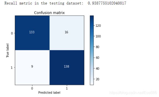
lr = LogisticRegression(C = best_c, penalty = 'l1',solver='liblinear')
lr.fit(X_train_undersample,y_train_undersample.values.ravel())
y_pred_undersample = lr.predict(X_test_undersample.values)

# Compute confusion matrix
cnf_matrix = confusion_matrix(y_test_undersample,y_pred_undersample)
np.set_printoptions(precision=2)

print("Recall metric in the testing dataset: ", cnf_matrix[1,1]/(cnf_matrix[1,0]+cnf_matrix[1,1]))

# Plot non-normalized confusion matrix
class_names = [0,1]
plt.figure()
plot_confusion_matrix(cnf_matrix
                      , classes=class_names
                      , title='Confusion matrix')
plt.show()

（8）在原始数据集上进行测试

lr = LogisticRegression(C = best_c, penalty = 'l1',solver='liblinear')
lr.fit(X_train_undersample,y_train_undersample.values.ravel())
y_pred = lr.predict(X_test.values) #原始测试集

# Compute confusion matrix
cnf_matrix = confusion_matrix(y_test,y_pred)
np.set_printoptions(precision=2)

print("Recall metric in the testing dataset: ", cnf_matrix[1,1]/(cnf_matrix[1,0]+cnf_matrix[1,1]))

# Plot non-normalized confusion matrix
class_names = [0,1]
plt.figure()
plot_confusion_matrix(cnf_matrix
                      , classes=class_names
                      , title='Confusion matrix')
plt.show()

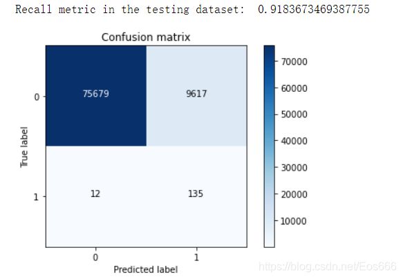
可以看到预测为1实际为0的样本数有9617个，这个值得大小不影响召回率，但从实际角度考虑会增加工作量，明明只有135个异常数据，但是模型却将很多正常数据误判为异常，这也是下采样存在得潜在问题，会有误杀现象！
（9）人为设定阈值，观察混淆矩阵

lr = LogisticRegression(C = 0.01, penalty = 'l1',solver='liblinear')
lr.fit(X_train_undersample,y_train_undersample.values.ravel())
y_pred_undersample_proba = lr.predict_proba(X_test_undersample.values) #预测概率值

thresholds = [0.1,0.2,0.3,0.4,0.5,0.6,0.7,0.8,0.9] #人为指定阈值

plt.figure(figsize=(10,10))

j = 1
for i in thresholds:
    y_test_predictions_high_recall = y_pred_undersample_proba[:,1] > i
    
    plt.subplot(3,3,j)
    j += 1
    
    # Compute confusion matrix
    cnf_matrix = confusion_matrix(y_test_undersample,y_test_predictions_high_recall)
    np.set_printoptions(precision=2)

    print("Recall metric in the testing dataset: ", cnf_matrix[1,1]/(cnf_matrix[1,0]+cnf_matrix[1,1]))

    # Plot non-normalized confusion matrix
    class_names = [0,1]
    plot_confusion_matrix(cnf_matrix
                          , classes=class_names
                          , title='Threshold >= %s'%i) 

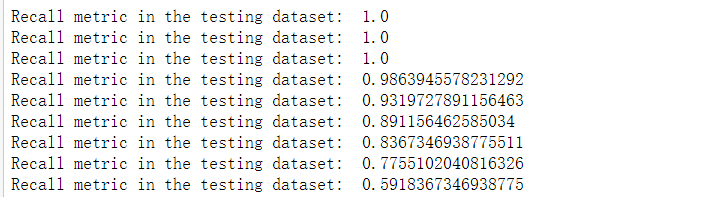
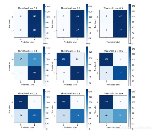当阈值设定为0.1，0.2，0.3时，可以看到预测值大部分都为1，说明判定太过严苛，虽然召回率为1，但实际出现很多误判。
当阈值设定0.4时，可有看到FN为92，表明存在大量误杀，（为了找到那异常得145个样本，模型把92个正常样本误杀为异常样本），虽然召回率为0.98，但实际效果依然不佳。
综上，我们应当选择合适得组合模型评估指标，选定效果最佳得模型。

4.利用过采样处理数据并进行模型训练

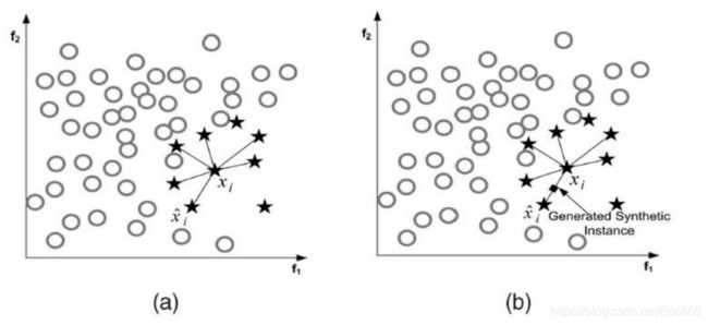
（1）SMOTE算法


（２）代码实现

import pandas as pd
from imblearn.over_sampling import SMOTE
from sklearn.ensemble import RandomForestClassifier
from sklearn.metrics import confusion_matrix
from sklearn.model_selection import train_test_split
credit_cards=pd.read_csv('creditcard.csv')

columns=credit_cards.columns
# The labels are in the last column ('Class'). Simply remove it to obtain features columns
features_columns=columns.delete(len(columns)-1)

features=credit_cards[features_columns]
labels=credit_cards['Class']
features_train, features_test, labels_train, labels_test = train_test_split(features, 
                                                                            labels, 
                                                                            test_size=0.2, 
                                                                            random_state=0)
oversampler=SMOTE(random_state=0)
os_features,os_labels=oversampler.fit_resample(features_train,labels_train)

os_features = pd.DataFrame(os_features)
os_labels = pd.DataFrame(os_labels)
best_c = printing_Kfold_scores(os_features,os_labels)
lr = LogisticRegression(C = best_c, penalty = 'l1')
lr.fit(os_features,os_labels.values.ravel())
y_pred = lr.predict(features_test.values)

# Compute confusion matrix
cnf_matrix = confusion_matrix(labels_test,y_pred)
np.set_printoptions(precision=2)

print("Recall metric in the testing dataset: ", cnf_matrix[1,1]/(cnf_matrix[1,0]+cnf_matrix[1,1]))

# Plot non-normalized confusion matrix
class_names = [0,1]
plt.figure()
plot_confusion_matrix(cnf_matrix
                      , classes=class_names
                      , title='Confusion matrix')
plt.show()

输出结果：

-------------------------------------------
C parameter:  0.01
-------------------------------------------

Iteration  1 : recall score =  0.8903225806451613
Iteration  2 : recall score =  0.8947368421052632
Iteration  3 : recall score =  0.9687506916011951
Iteration  4 : recall score =  0.9579252811026479
Iteration  5 : recall score =  0.9579472637144019

Mean recall score  0.9339365318337338

-------------------------------------------
C parameter:  0.1
-------------------------------------------

Iteration  1 : recall score =  0.8903225806451613
Iteration  2 : recall score =  0.8947368421052632
Iteration  3 : recall score =  0.9704326657076463
Iteration  4 : recall score =  0.9595410030665743
Iteration  5 : recall score =  0.9606511249601565

Mean recall score  0.9351368432969602

-------------------------------------------
C parameter:  1
-------------------------------------------

Iteration  1 : recall score =  0.8903225806451613
Iteration  2 : recall score =  0.8947368421052632
Iteration  3 : recall score =  0.9704547969458891
Iteration  4 : recall score =  0.9605082379837548
Iteration  5 : recall score =  0.960112550972181

Mean recall score  0.9352270017304498

-------------------------------------------
C parameter:  10
-------------------------------------------

Iteration  1 : recall score =  0.8903225806451613
Iteration  2 : recall score =  0.8947368421052632
Iteration  3 : recall score =  0.9705433218988603
Iteration  4 : recall score =  0.9601455248898122
Iteration  5 : recall score =  0.9608050032424352

Mean recall score  0.9353106545563064

-------------------------------------------
C parameter:  100
-------------------------------------------

Iteration  1 : recall score =  0.8903225806451613
Iteration  2 : recall score =  0.8947368421052632
Iteration  3 : recall score =  0.9704769281841319
Iteration  4 : recall score =  0.9599916466075334
Iteration  5 : recall score =  0.9601675075015662

Mean recall score  0.9351391010087312

*********************************************************************************
Best model to choose from cross validation is with C parameter =  10.0
*********************************************************************************

可以看到误杀明显减少，并且召回率较高。

---