机器学习笔记-逻辑回归实战案例-信用卡欺诈检测

机器学习笔记-逻辑回归实战案例-信用卡欺诈检测

基于creditcard.csv实现数据，建立逻辑回归模型，对数据进行分类

---

手码不易，点波关注呗

环境：python 3.7.5 and pycharm 2020.1.2

---

前言

字数：15871阅读时间：30 mins

---

提示：以下是本篇文章正文内容，下面案例可供参考

一、数据分析与预处理

数据读取与分析

没有安装模块的先安装模块啦！！

1.数据读取与分析

这是全局的一个模块工具需要，先剧透一波

################数据分析模块导入######################
import pandas as pd
import numpy as np
import matplotlib.pyplot as plt
from sklearn.preprocessing import StandardScaler # 导入sklearn标准化模块
from sklearn.model_selection import train_test_split # 数据集合拆分模块
from sklearn.model_selection import KFold
from sklearn.linear_model import LogisticRegression
from sklearn.metrics import recall_score
from sklearn.metrics import confusion_matrix
import itertools
from imblearn.over_sampling import SMOTE

################数据读取######################
data = pd.read_csv('creditcard.csv')
print(data.head(2))
print(data.info())

代码结果：

   Time        V1        V2        V3  ...       V27       V28  Amount  Class
0   0.0 -1.359807 -0.072781  2.536347  ...  0.133558 -0.021053  149.62      0
1   0.0  1.191857  0.266151  0.166480  ... -0.008983  0.014724    2.69      0

<class 'pandas.core.frame.DataFrame'>
RangeIndex: 284807 entries, 0 to 284806
Data columns (total 31 columns):
 #   Column  Non-Null Count   Dtype  
---  ------  --------------   -----  
 0   Time    284807 non-null  float64
 1   V1      284807 non-null  float64
 2   V2      284807 non-null  float64
 3   V3      284807 non-null  float64
 4   V4      284807 non-null  float64
 5   V5      284807 non-null  float64
 6   V6      284807 non-null  float64
 7   V7      284807 non-null  float64
 8   V8      284807 non-null  float64
 9   V9      284807 non-null  float64
 10  V10     284807 non-null  float64
 11  V11     284807 non-null  float64
 12  V12     284807 non-null  float64
 13  V13     284807 non-null  float64
 14  V14     284807 non-null  float64
 15  V15     284807 non-null  float64
 16  V16     284807 non-null  float64
 17  V17     284807 non-null  float64
 18  V18     284807 non-null  float64
 19  V19     284807 non-null  float64
 20  V20     284807 non-null  float64
 21  V21     284807 non-null  float64
 22  V22     284807 non-null  float64
 23  V23     284807 non-null  float64
 24  V24     284807 non-null  float64
 25  V25     284807 non-null  float64
 26  V26     284807 non-null  float64
 27  V27     284807 non-null  float64
 28  V28     284807 non-null  float64
 29  Amount  284807 non-null  float64
 30  Class   284807 non-null  int64  
dtypes: float64(30), int64(1)
memory usage: 67.4 MB

creditcard.csv数据获取，关注博主，传送门
共31列，没有特征解释，显得十分的纯粹。
Amount贷款金额，Class分类结果，其中0表示正常，1表示异常

# 观察正常与异常数据
count_classes = pd.value_counts(data['Class'],sort=True).sort_index()
count_classes.plot(kind = 'bar')
plt.title('Fraud class histogram')
plt.xlabel('Class')
plt.ylabel('Frequency')

plt.show()

通过简单的观察画图，看出正常数据与异常数据的比例大小，是否均衡？
Answers:False

2.样本不均衡解决方案

（1）下采样：通俗讲-假设异常数据500个，正常数据100000个，取正常500个
（2）过采样：通俗讲-假设异常数据500个，正常数据100000个，造999500个异常数据

样本不均衡解决方法

标准化

考虑到Amount数据相对其他数据差异较大，采用特征标准化，公式如下：

特征标准化

###############数据标准化######################
data['normAmount'] = StandardScaler().fit_transform(data['Amount'].values.reshape(-1,1))
data = data.drop(['Time','Amount'],axis=1) # 删除2列
print(data.head(5))

结果展示：

         V1        V2        V3  ...       V28  Class  normAmount
0 -1.359807 -0.072781  2.536347  ... -0.021053      0    0.244964
1  1.191857  0.266151  0.166480  ...  0.014724      0   -0.342475
2 -1.358354 -1.340163  1.773209  ... -0.059752      0    1.160686
3 -0.966272 -0.185226  1.792993  ...  0.061458      0    0.140534
4 -1.158233  0.877737  1.548718  ...  0.215153      0   -0.073403

[5 rows x 30 columns]
正常样本比例： 0.5
异常样本比例： 0.5
下采样总样本数： 984

注意：pandas的reshape一般是传入元组，但是，这里reshape(-1,1)是将心的数据转换成一列

二、下采样方案

##################数据下采样#############
# 目的是获得与异常样本一样多的数据
# 不包含标签的就是特征
x = data.loc[:,data.columns != 'Class']
# 标签
y = data.loc[:,data.columns == 'Class']
number_records_fraud = len(data[data.Class == 1])
# 得到异常样本的索引
fraud_indices = np.array(data[data.Class == 1].index)
# 得到所有正常样本的索引
normal_indices = data[data.Class == 0].index
# https://blog.csdn.net/qq1483661204/article/details/77587881 索引的运用
# 从正常样本中随机抽样指定个数的样本，并取其索引
random_normal_indices = np.random.choice(normal_indices,number_records_fraud,replace=False)
random_normal_indices = np.array(random_normal_indices)
# 有了正常和异常的样本后把他们的索引都拿到手
under_sample_indices = np.concatenate([fraud_indices,random_normal_indices])

# 根据索引得到下采样的所有样本量
under_sample_data = data.iloc[under_sample_indices,:]
x_undersample = under_sample_data.loc[:, under_sample_data.columns !='Class']
y_undersample = under_sample_data.loc[:,under_sample_data.columns == 'Class']

# 打印下采样策略后正负样本比例
print('正常样本比例：',len(under_sample_data[under_sample_data.Class == 0])/len(under_sample_data))
print('异常样本比例：',len(under_sample_data[under_sample_data.Class == 1])/len(under_sample_data))
print('下采样总样本数：',len(under_sample_data))

结果展示：

正常样本比例： 0.5
异常样本比例： 0.5
下采样总样本数： 984

1.交叉验证

什么是交叉验证？
我也显得十分困惑，先看一个图（百度图片）

举个例子：将分出来的测试集，在分为10份，第一次将取9份，留一份作为验证集；第二次，还是取9份，在留其他的一份作为验证集，循环10次。得到10次的计算结果，计算平均数，得到最终模型的评估结果。以上过程，就是交叉验证

###################交叉验证###############################

# 导入数据集切分模块

x_train,x_test,y_train, y_test = train_test_split(x,y,test_size = 0.3,random_state=0)
# 划分数据集，x为特征，y为标签，test_size为测试集比例，random_state设置随机种子
print('原始训练集包含样本数量：',len(x_train))
print('原始测试训练集样本数量：',len(x_test))
print('原始样本样本数量：',len(x_train)+len(x_test))

# 下采样数据集进行划分
x_train_undersample,x_test_undersample,y_train_undersample,y_test_undersample = train_test_split(x_undersample,y_undersample, random_state=0, test_size=0.3)
print('原始训练集包含样本数量：',len(x_train_undersample))
print('原始测试训练集样本数量：',len(x_test_undersample))
print('原始样本样本数量：',len(x_train_undersample)+len(x_test_undersample))

代码结果：

原始训练集包含样本数量： 199364
原始测试训练集样本数量： 85443
原始样本样本数量： 284807
原始训练集包含样本数量： 688
原始测试训练集样本数量： 296
原始样本样本数量： 984

2.模型评估方法

模型评估的真真假假？？？

百度图片，模糊凑合看
T：True，F：False P：Position N：negative

	相关（Relevant）正类	无关（No-Relevant）负类
被检索到（Retrieved）	TP：预测正确，判为正类	FP：预测错误，判为正类 （存伪）
未被检索到（No-Retrieved）	FN：预测错误，判为负类 （去真）	TN：预测正确，判为负类

3种常见的评估指标

准确率（accuracy）：分类正确的占总的比例

召回率（recall）：分类正确且判为正类占所有正类的比例

精确度（precision）：分类正确占所有判为正类的比例

3.正则化惩罚

不禁要问：为什么要惩罚呢？
模型拟合有欠拟合、正常拟合、过拟合，过拟合调皮（模型拟合度较高，虽然对训练集比较好，但是一旦实际测试，一塌糊涂），所以要惩罚：
继续问：怎么惩罚呢？
对参数赋予一定权重。常见有L1，L2正则化惩罚项

逻辑回归模型

1.参数对结果的影响

MD，终于开始建模了！
直接上代码，我等不及了！

#################逻辑回归模型######################
def printing_Kflod_scores(x_train_data,y_train_data):
    fold = KFold(5,shuffle=False) # len(y_train_data),删除
    # 定义不用的正则化惩罚力度
    c_param_range = [0.01,0.1,1,10,100]
    # 展示结果用的表格
    results_table = pd.DataFrame(index = range(len(c_param_range),2),columns=['C_parameter','Mean recall score'])
    results_table['C_parameter']  = c_param_range
    # k-flod表示K折交叉验证，这里会得到两个索引集合：训练集= indices[0],验证集=indices[1]
    j = 0
    # 循环遍历不同参数
    for c_param in c_param_range:
        print('-'*30)
        print('正则化惩罚力度：',c_param)
        print('-' * 30)
        print('')
        recall_accs = []
        # 分解来执行交叉验证
        for iteration,indices in enumerate(fold.split(x_train_data)):
            # 指定算法模型，给定参数
            lr = LogisticRegression(C=c_param,penalty = 'l1',solver='liblinear')
            # 训练模型，主要不要给错索引，训练的一定是训练集，所以x，y的所有都是0
            lr.fit(x_train_data.iloc[indices[0],:],y_train_data.iloc[indices[0],:].values.ravel())
            # 测试，预测模型效果，用到验证集，索引为1
            y_pred_undersample = lr.predict(x_train_data.iloc[indices[1],:].values)
            # 预测结果后，进行模型评估，这里用recall_score需要传入预测值和真实值
            recall_acc = recall_score(y_train_data.iloc[indices[1],:].values,y_pred_undersample)
            # 还要计算平均，先保存结果
            recall_accs.append(recall_acc)
            print('Iteration',iteration,':召回率 = ',recall_acc)
        # 当执行完所有交叉验证后，计算平均结果
        results_table.loc[j,'Mean recall score'] = np.mean(recall_accs)
        j += 1
        print('')
        print('平均召回率：',np.mean(recall_accs))
        print('')
        # 找到参数最好的，也就是recall最高的
        best_c = results_table.loc[results_table['Mean recall score'].astype('float32').idxmax()]['C_parameter']

    # 打印出最好的结果
    print('-'*30)
    print('效果最好的模型所选的参数：',best_c)
    print('-'*30)
    print(results_table)
    return best_c
# 函数调用
best_c = printing_Kflod_scores(x_train_undersample,y_train_undersample)
# 在sklearn中惩罚力度，取决于参数C，数值越小，惩罚力度越大。

代码结果：

------------------------------
正则化惩罚力度： 0.01
------------------------------

Iteration 0 :召回率 =  0.9315068493150684
Iteration 1 :召回率 =  0.9178082191780822
Iteration 2 :召回率 =  1.0
Iteration 3 :召回率 =  0.9594594594594594
Iteration 4 :召回率 =  0.9696969696969697

平均召回率： 0.955694299529916

------------------------------
正则化惩罚力度： 0.1
------------------------------

Iteration 0 :召回率 =  0.8493150684931506
Iteration 1 :召回率 =  0.863013698630137
Iteration 2 :召回率 =  0.9491525423728814
Iteration 3 :召回率 =  0.9459459459459459
Iteration 4 :召回率 =  0.8787878787878788

平均召回率： 0.8972430268459988

------------------------------
正则化惩罚力度： 1
------------------------------

Iteration 0 :召回率 =  0.863013698630137
Iteration 1 :召回率 =  0.8904109589041096
Iteration 2 :召回率 =  0.9830508474576272
Iteration 3 :召回率 =  0.9459459459459459
Iteration 4 :召回率 =  0.9090909090909091

平均召回率： 0.9183024720057457

------------------------------
正则化惩罚力度： 10
------------------------------

Iteration 0 :召回率 =  0.863013698630137
Iteration 1 :召回率 =  0.8904109589041096
Iteration 2 :召回率 =  0.9830508474576272
Iteration 3 :召回率 =  0.9324324324324325
Iteration 4 :召回率 =  0.9090909090909091

平均召回率： 0.9155997693030431

------------------------------
正则化惩罚力度： 100
------------------------------

Iteration 0 :召回率 =  0.863013698630137
Iteration 1 :召回率 =  0.8904109589041096
Iteration 2 :召回率 =  0.9830508474576272
Iteration 3 :召回率 =  0.9459459459459459
Iteration 4 :召回率 =  0.9090909090909091

平均召回率： 0.9183024720057457

------------------------------
效果最好的模型所选的参数： 0.01
------------------------------

注意：C=0.01表示正则化力度，随着数值的增加，惩罚力度是减小的。

2.混淆矩阵

混淆矩阵，真头大，简化表述就是：就是TP、FP、FN、TN的统计个数形成的2X2维矩阵

画一画

###############混淆矩阵####################
#　作用：更直观展现结果

def plot_confusion_matrix(cm,classes,title='Confusion Matrix',cmap=plt.cm.Reds):
    plt.imshow(cm,interpolation='nearest',cmap = cmap)
    plt.title(title)
    plt.colorbar()
    tick_marks = np.arange(len(classes))
    plt.xticks(tick_marks,classes,rotation=0)
    plt.yticks(tick_marks,classes)

    thresh = cm.max()/2
    for i , j in itertools.product(range(cm.shape[0]),range(cm.shape[1])):
        plt.text(j,i,cm[i,j],
                 horizontalalignment='center',
                 color='white' if cm[i,j] > thresh else 'black')

    plt.tight_layout()
    plt.ylabel('True label')
    plt.xlabel('Predicted label')

# 下采样传值
lr = LogisticRegression(C = best_c,penalty='l1',solver='liblinear')
lr.fit(x_train_undersample,y_train_undersample.values.ravel())
y_pred_undersample = lr.predict(x_test_undersample.values)
# 计算所需的值
cnf_matrix = confusion_matrix(y_test_undersample,y_pred_undersample)
np.set_printoptions(precision=2)
print('召回率：',cnf_matrix[1,1]/(cnf_matrix[1,0]+cnf_matrix[1,1]))
# 绘图
class_names = [0,1]
plt.figure()
plot_confusion_matrix(cnf_matrix,classes=class_names,title='Confusion matrix')
plt.show()

#　原始数据传值
lr = LogisticRegression(C = best_c,penalty='l1',solver='liblinear')
lr.fit(x_train_undersample,y_train_undersample.values.ravel())
y_pred = lr.predict(x_test.values)
# 计算所需的值
cnf_matrix = confusion_matrix(y_test,y_pred)
np.set_printoptions(precision=2)
print('Recall metric in the testing dataset：',cnf_matrix[1,1]/(cnf_matrix[1,0]+cnf_matrix[1,1]))
# 绘图
class_names = [0,1]
plt.figure()
plot_confusion_matrix(cnf_matrix,classes=class_names,title='Confusion matrix')

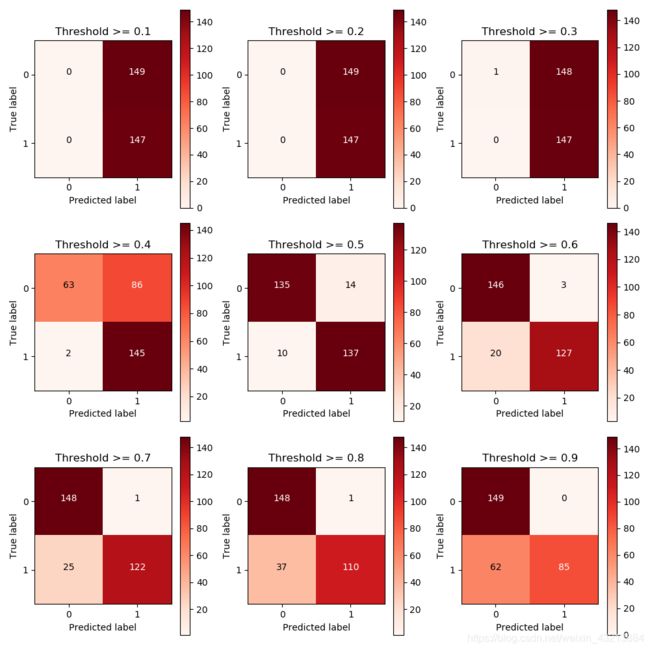
3.分类阈值对结果的影响

分类阈值是个什么东西？？？
就是把一个样本数据判为一类的概率值，经验是0.5

#####################分类与之对结果的影响########################
# 用之前最好的参数来进行建模
lr = LogisticRegression(C = 0.01,penalty='l1',solver='liblinear')
lr.fit(x_train_undersample,y_train_undersample.values.ravel())
y_pred_undersample_proba = lr.predict_proba(x_test_undersample.values)
# 指定不同的阈值
thresholds = [0.1,0.2,0.3,0.4,0.5,0.6,0.7,0.8,0.9]
plt.figure(figsize=(10,10))
j = 1
# 用混淆矩阵来进行展示
for i in thresholds:
    # 比较预测概率和给定的阈值
    y_test_predictions_high_recall = y_pred_undersample_proba[:,1] > i
    plt.subplot(3,3,j)
    j += 1
    cnf_matrix = confusion_matrix(y_test_undersample,y_test_predictions_high_recall)
    np.set_printoptions(precision=2)
    print('Recall metric in the testing dataset:',cnf_matrix[1,1]/(cnf_matrix[1,0]+cnf_matrix[1,1]))    
    class_names = [0,1]
    plot_confusion_matrix(cnf_matrix,classes=class_names,title='Threshold >= %s'%i)

Recall metric in the testing dataset： 0.9183673469387755
Recall metric in the testing dataset: 1.0
Recall metric in the testing dataset: 1.0
Recall metric in the testing dataset: 1.0
Recall metric in the testing dataset: 0.9863945578231292
Recall metric in the testing dataset: 0.9319727891156463
Recall metric in the testing dataset: 0.8639455782312925
Recall metric in the testing dataset: 0.8299319727891157
Recall metric in the testing dataset: 0.7482993197278912
Recall metric in the testing dataset: 0.5782312925170068

当阈值在0.5时，召回率偏高，误判样本也明显较多。
当阈值在0.6时，召回率有所下降，误判样本也明显减少。
选谁呢？诶！根据业务需求！

过采样方法

1.SMOTE数据生成策略

为什么要SMOTE，我们看前面的结果，虽然召回率较高，但是误判的样本也不少
大概思路：
对每一个异常样本，首先找到（欧氏距离）最近的同类样本，然后在他们之间的举例之上取0-1中的一个随机小数作为比例，在加到原始数据点，就得到最新的异常样本。

2.过采样应用效果

#############SMOTE数据生成策略###############
# pip install imblearn
features_train, features_test, labels_train, labels_test = train_test_split(x,
                                                                            y,
                                                                            test_size=0.3,
                                                                            random_state=0)
oversampler = SMOTE(random_state=0)
os_features,os_labels = oversampler.fit_sample(features_train,labels_train)

os_features = pd.DataFrame(os_features)
os_labels = pd.DataFrame(os_labels)
best_c = printing_Kflod_scores(os_features,os_labels)

lr = LogisticRegression(C = best_c,penalty='l1',solver='liblinear')
lr.fit(os_features,os_labels.values.ravel())
y_pred = lr.predict(features_test.values)
# 计算混淆矩阵
cnf_matrix = confusion_matrix(labels_test,y_pred)
np.set_printoptions(precision=2)
print('Recall metric in the testing dataset:', cnf_matrix[1, 1] / (cnf_matrix[1, 0] + cnf_matrix[1, 1]))
class_names = [0, 1]
plt.figure()
plot_confusion_matrix(cnf_matrix, classes=class_names, title='Confusion matrix')

plt.show()

结果展示：

------------------------------
正则化惩罚力度： 0.01
------------------------------

Iteration 0 :召回率 =  0.9285714285714286
Iteration 1 :召回率 =  0.912
Iteration 2 :召回率 =  0.9129742033383915
Iteration 3 :召回率 =  0.897245217129147
Iteration 4 :召回率 =  0.8974336427701082

平均召回率： 0.9096448983618151

------------------------------
正则化惩罚力度： 0.1
------------------------------

Iteration 0 :召回率 =  0.9285714285714286
Iteration 1 :召回率 =  0.92
Iteration 2 :召回率 =  0.9145169448659585
Iteration 3 :召回率 =  0.8985139497782858
Iteration 4 :召回率 =  0.8987777456756315

平均召回率： 0.9120760137782609

------------------------------
正则化惩罚力度： 1
------------------------------

Iteration 0 :召回率 =  0.9285714285714286
Iteration 1 :召回率 =  0.92
Iteration 2 :召回率 =  0.914693980778958
Iteration 3 :召回率 =  0.8988028690944264
Iteration 4 :召回率 =  0.8990917884105669

平均召回率： 0.9122320133710762

------------------------------
正则化惩罚力度： 10
------------------------------

Iteration 0 :召回率 =  0.9285714285714286
Iteration 1 :召回率 =  0.92
Iteration 2 :召回率 =  0.914693980778958
Iteration 3 :召回率 =  0.8991294735387592
Iteration 4 :召回率 =  0.8991169118293617

平均召回率： 0.9123023589437016

------------------------------
正则化惩罚力度： 100
------------------------------

Iteration 0 :召回率 =  0.9285714285714286
Iteration 1 :召回率 =  0.92
Iteration 2 :召回率 =  0.9146686899342438
Iteration 3 :召回率 =  0.8990917884105669
Iteration 4 :召回率 =  0.8991169118293617

平均召回率： 0.9122897637491203

------------------------------
效果最好的模型所选的参数： 10.0
------------------------------
   C_parameter Mean recall score
0         0.01          0.909645
1         0.10          0.912076
2         1.00          0.912232
3        10.00          0.912302
4       100.00           0.91229
Recall metric in the testing dataset: 0.9183673469387755

Process finished with exit code 0