机器学习笔记 - 使用TensorFlow2.0 + ResNet进行疟疾预测

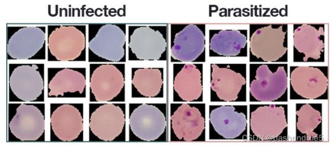
 一、疟疾数据库（血液样本的图片）

        数据集下载地址，美国国立卫生研究院网站

LHNCBC Full Download Listhttps://ceb.nlm.nih.gov/repositories/malaria-datasets/

        该数据集由属于两个不同类别的 27,588 张图像组成。每个类别的图像数量均等分布，每个类别有 13,794 张图像。

1. 寄生：暗示该地区含有疟疾。
2. 未感染：意味着该地区没有疟疾的证据。 

美国国立卫生研究院 (NIH) 提供的疟疾数据集的一个子集。我们将使用该数据集使用 Python、OpenCV 和 Keras 开发深度学习医学影像分类模型。

        美国国立卫生研究院使用了六个预训练的卷积神经网络，如下，最终得到了95.9%的准确率。

        AlexNet

        VGG-16

        ResNet-50

        Xception

        DenseNet-121

        A customized model they created

        美国国立卫生研究院网站上提供了自定义的网络模型和DenseNet-121的网络模型的源码。

        我们这里使用resnet进行训练。 

二、组织代码

1、resnet.py，resnet模型

# import the necessary packages
from tensorflow.keras.layers import BatchNormalization
from tensorflow.keras.layers import Conv2D
from tensorflow.keras.layers import AveragePooling2D
from tensorflow.keras.layers import MaxPooling2D
from tensorflow.keras.layers import ZeroPadding2D
from tensorflow.keras.layers import Activation
from tensorflow.keras.layers import Dense
from tensorflow.keras.layers import Flatten
from tensorflow.keras.layers import Input
from tensorflow.keras.models import Model
from tensorflow.keras.layers import add
from tensorflow.keras.regularizers import l2
from tensorflow.keras import backend as K

class ResNet:
    @staticmethod
    def residual_module(data, K, stride, chanDim, red=False, reg=0.0001, bnEps=2e-5, bnMom=0.9):
        # the shortcut branch of the ResNet module should be
        # initialize as the input (identity) data
        shortcut = data
        # the first block of the ResNet module are the 1x1 CONVs
        bn1 = BatchNormalization(axis=chanDim, epsilon=bnEps, momentum=bnMom)(data)
        act1 = Activation("relu")(bn1)
        conv1 = Conv2D(int(K * 0.25), (1, 1), use_bias=False, kernel_regularizer=l2(reg))(act1)

        # the second block of the ResNet module are the 3x3 CONVs
        bn2 = BatchNormalization(axis=chanDim, epsilon=bnEps, momentum=bnMom)(conv1)
        act2 = Activation("relu")(bn2)
        conv2 = Conv2D(int(K * 0.25), (3, 3), strides=stride, padding="same", use_bias=False, kernel_regularizer=l2(reg))(act2)

        # the third block of the ResNet module is another set of 1x1
        # CONVs
        bn3 = BatchNormalization(axis=chanDim, epsilon=bnEps, momentum=bnMom)(conv2)
        act3 = Activation("relu")(bn3)
        conv3 = Conv2D(K, (1, 1), use_bias=False, kernel_regularizer=l2(reg))(act3)

        # if we are to reduce the spatial size, apply a CONV layer to
        # the shortcut
        if red:
            shortcut = Conv2D(K, (1, 1), strides=stride, use_bias = False, kernel_regularizer = l2(reg))(act1)

        # add together the shortcut and the final CONV
        x = add([conv3, shortcut])
        # return the addition as the output of the ResNet module
        return x

    @ staticmethod
    def build(width, height, depth, classes, stages, filters, reg=0.0001, bnEps=2e-5, bnMom=0.9, dataset="cifar"):
        # initialize the input shape to be "channels last" and the
        # channels dimension itself
        inputShape = (height, width, depth)
        chanDim = -1
        # if we are using "channels first", update the input shape
        # and channels dimension
        if K.image_data_format() == "channels_first":
            inputShape = (depth, height, width)
            chanDim = 1

        # set the input and apply BN
        inputs = Input(shape=inputShape)
        x = BatchNormalization(axis=chanDim, epsilon=bnEps, momentum = bnMom)(inputs)
        # check if we are utilizing the CIFAR dataset
        if dataset == "cifar":
            # apply a single CONV layer
            x = Conv2D(filters[0], (3, 3), use_bias=False, padding = "same", kernel_regularizer = l2(reg))(x)

        # loop over the number of stages
        for i in range(0, len(stages)):
            # initialize the stride, then apply a residual module
            # used to reduce the spatial size of the input volume
            stride = (1, 1) if i == 0 else (2, 2)
            x = ResNet.residual_module(x, filters[i + 1], stride, chanDim, red=True, bnEps=bnEps, bnMom=bnMom)

            # loop over the number of layers in the stage
            for j in range(0, stages[i] - 1):
                x = ResNet.residual_module(x, filters[i + 1], (1, 1), chanDim, bnEps=bnEps, bnMom=bnMom)

        # apply BN => ACT => POOL
        x = BatchNormalization(axis=chanDim, epsilon=bnEps, momentum = bnMom)(x)
        x = Activation("relu")(x)
        x = AveragePooling2D((8, 8))(x)
        # softmax classifier
        x = Flatten()(x)
        x = Dense(classes, kernel_regularizer=l2(reg))(x)
        x = Activation("softmax")(x)

        # create the model
        model = Model(inputs, x, name="resnet")

        # return the constructed network architecture
        return model

2、config.py，配置文件

# import the necessary packages
import os
# initialize the path to the *original* input directory of images
# 下载的数据集的路径
ORIG_INPUT_DATASET = "cell_images"
# initialize the base path to the *new* directory that will contain
# our images after computing the training and testing split
BASE_PATH = "malaria"
# derive the training, validation, and testing directories
TRAIN_PATH = os.path.sep.join([BASE_PATH, "training"])
VAL_PATH = os.path.sep.join([BASE_PATH, "validation"])
TEST_PATH = os.path.sep.join([BASE_PATH, "testing"])
# define the amount of data that will be used training
TRAIN_SPLIT = 0.8
# the amount of validation data will be a percentage of the
# *training* data
VAL_SPLIT = 0.1

3、构建数据集，build_dataset.py

        我们的疟疾数据集没有用于训练、验证和测试的预拆分数据，因此我们需要自己执行拆分。

        要创建我们的数据拆分，我们将创建build_dataset.py脚本——这个脚本将：

        1、获取我们所有示例图像的路径并随机打乱它们。

        2、将图像路径拆分为训练、验证和测试。

        3、新建三个子目录 疟疾/ 目录，即 训练、验证和测试。

        4、自动将图像复制到其对应的目录中。

# import the necessary packages
import config
from imutils import paths
import random
import shutil
import os
# grab the paths to all input images in the original input directory
# and shuffle them
imagePaths = list(paths.list_images(config.ORIG_INPUT_DATASET))
random.seed(42)
random.shuffle(imagePaths)

# compute the training and testing split
i = int(len(imagePaths) * config.TRAIN_SPLIT)
trainPaths = imagePaths[:i]
testPaths = imagePaths[i:]
# we'll be using part of the training data for validation
i = int(len(trainPaths) * config.VAL_SPLIT)
valPaths = trainPaths[:i]
trainPaths = trainPaths[i:]

# define the datasets that we'll be building
datasets = [
	("training", trainPaths, config.TRAIN_PATH),
	("validation", valPaths, config.VAL_PATH),
	("testing", testPaths, config.TEST_PATH)
]

# loop over the datasets
for (dType, imagePaths, baseOutput) in datasets:
	# show which data split we are creating
	print("[INFO] building '{}' split".format(dType))
	# if the output base output directory does not exist, create it
	if not os.path.exists(baseOutput):
		print("[INFO] 'creating {}' directory".format(baseOutput))
		os.makedirs(baseOutput)
	# loop over the input image paths
	for inputPath in imagePaths:
		# extract the filename of the input image along with its
		# corresponding class label
		filename = inputPath.split(os.path.sep)[-1]
		label = inputPath.split(os.path.sep)[-2]
		# build the path to the label directory
		labelPath = os.path.sep.join([baseOutput, label])
		# if the label output directory does not exist, create it
		if not os.path.exists(labelPath):
			print("[INFO] 'creating {}' directory".format(labelPath))
			os.makedirs(labelPath)
		# construct the path to the destination image and then copy
		# the image itself
		p = os.path.sep.join([labelPath, filename])
		shutil.copy2(inputPath, p)

4、训练模型，train_model.py

# set the matplotlib backend so figures can be saved in the background
import matplotlib
matplotlib.use("Agg")
# import the necessary packages
from tensorflow.keras.preprocessing.image import ImageDataGenerator
from tensorflow.keras.callbacks import LearningRateScheduler
from tensorflow.keras.optimizers import SGD
from models.resnet.resnet import ResNet
import config
from sklearn.metrics import classification_report
from imutils import paths
import matplotlib.pyplot as plt
import numpy as np
import argparse
# construct the argument parser and parse the arguments
ap = argparse.ArgumentParser()
ap.add_argument("-p", "--plot", type=str, default="plot.png",
	help="path to output loss/accuracy plot")
args = vars(ap.parse_args())

# define the total number of epochs to train for along with the
# initial learning rate and batch size
NUM_EPOCHS = 50
INIT_LR = 1e-1
BS = 32

def poly_decay(epoch):
	# initialize the maximum number of epochs, base learning rate,
	# and power of the polynomial
	maxEpochs = NUM_EPOCHS
	baseLR = INIT_LR
	power = 1.0
	# compute the new learning rate based on polynomial decay
	alpha = baseLR * (1 - (epoch / float(maxEpochs))) ** power
	# return the new learning rate
	return alpha

# determine the total number of image paths in training, validation,
# and testing directories
totalTrain = len(list(paths.list_images(config.TRAIN_PATH)))
totalVal = len(list(paths.list_images(config.VAL_PATH)))
totalTest = len(list(paths.list_images(config.TEST_PATH)))

# initialize the training training data augmentation object
trainAug = ImageDataGenerator(
	rescale=1 / 255.0,
	rotation_range=20,
	zoom_range=0.05,
	width_shift_range=0.05,
	height_shift_range=0.05,
	shear_range=0.05,
	horizontal_flip=True,
	fill_mode="nearest")
# initialize the validation (and testing) data augmentation object
valAug = ImageDataGenerator(rescale=1 / 255.0)

# initialize the training generator
trainGen = trainAug.flow_from_directory(
	config.TRAIN_PATH,
	class_mode="categorical",
	target_size=(64, 64),
	color_mode="rgb",
	shuffle=True,
	batch_size=BS)
# initialize the validation generator
valGen = valAug.flow_from_directory(
	config.VAL_PATH,
	class_mode="categorical",
	target_size=(64, 64),
	color_mode="rgb",
	shuffle=False,
	batch_size=BS)
# initialize the testing generator
testGen = valAug.flow_from_directory(
	config.TEST_PATH,
	class_mode="categorical",
	target_size=(64, 64),
	color_mode="rgb",
	shuffle=False,
	batch_size=BS)

# initialize our ResNet model and compile it
model = ResNet.build(64, 64, 3, 2, (3, 4, 6), (64, 128, 256, 512), reg=0.0005)
opt = SGD(lr=INIT_LR, momentum=0.9)
model.compile(loss="binary_crossentropy", optimizer=opt, metrics=["accuracy"])

# define our set of callbacks and fit the model
callbacks = [LearningRateScheduler(poly_decay)]
H = model.fit(
	x=trainGen,
	steps_per_epoch=totalTrain // BS,
	validation_data=valGen,
	validation_steps=totalVal // BS,
	epochs=NUM_EPOCHS,
	callbacks=callbacks)

# reset the testing generator and then use our trained model to
# make predictions on the data
print("[INFO] evaluating network...")
testGen.reset()
predIdxs = model.predict(x=testGen, steps=(totalTest // BS) + 1)
# for each image in the testing set we need to find the index of the
# label with corresponding largest predicted probability
predIdxs = np.argmax(predIdxs, axis=1)
# show a nicely formatted classification report
print(classification_report(testGen.classes, predIdxs, target_names=testGen.class_indices.keys()))

# plot the training loss and accuracy
N = NUM_EPOCHS
plt.style.use("ggplot")
plt.figure()
plt.plot(np.arange(0, N), H.history["loss"], label="train_loss")
plt.plot(np.arange(0, N), H.history["val_loss"], label="val_loss")
plt.plot(np.arange(0, N), H.history["accuracy"], label="train_acc")
plt.plot(np.arange(0, N), H.history["val_accuracy"], label="val_acc")
plt.title("Training Loss and Accuracy on Dataset")
plt.xlabel("Epoch #")
plt.ylabel("Loss/Accuracy")
plt.legend(loc="lower left")
plt.savefig(args["plot"])

5、训练结果

        每个epoch在单个 rtx2060 GPU 上大约 130 秒。在第 50 个时期结束时，我们在训练、验证和测试数据上获得了96% 的准确率。

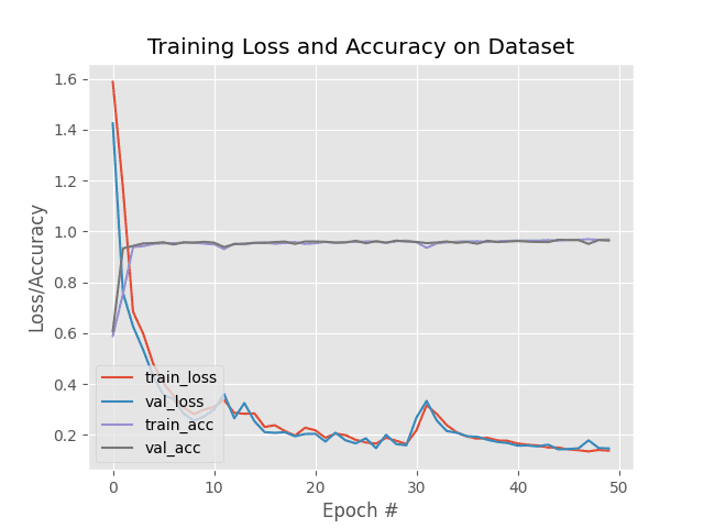训练/测试准确度和损失图表明我们已经实现了高准确度和低损失。该模型没有表现出过度/欠拟合的迹象。这种深度学习医学成像“疟疾分类器”模型是使用 Keras/TensorFlow 使用 ResNet 架构创建的。