Python计算机视觉编程第二章 局部图像描述子

1 Harris角点检测

1.1基本概念

Harris角点检测算法（也称Harris&Stephens角点检测器）是一个极为简单的交点检测算法。该算法的主要思想是，如果像素周围显示存在多于一个方向的边，我们认为该点为兴趣点。该点就称为角点。
我们把图像域中点x上的对称半正定矩阵MI=MI(x)定义为：

其中∇I为包含导数Ix和Iy的图像梯度。由于该定义，MI的秩为1，特征值为λ1=|∇I|2和λ2=0。现在对于图像的每个像素，我们可以计算出该矩阵。
选择权重矩阵W（通常为高斯滤波器Gσ），我们可以得到卷积：

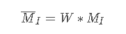
该卷积的目的是得到MI在周围像素上的局部平均。计算出的矩阵MI-有称为Harris矩阵。W的宽度决定了在像素x周围的感兴趣区域。像这样在区域附近对矩阵MI-取平均的原因是，特征值会依赖于局部图像特性而变化。如果图像梯度在该区域变化，那么MI-的第二个特征值将不再为0.如果图像的梯度没有变换，MI-的特征值也不会变化。
取决于该区域∇I的值，Harris矩阵MI-的特征值有三种情况：
1）如果λ1和λ2都是很大的正数，则该x点为角点；
2）如果λ1很大，λ2≈0，则该区域内存在一个边，该区域内的平均MI-的特征值不会变化太大；
3）如果λ1≈λ2≈0，则该区域为空。

为了去除加权常数κ，我们通常使用商数

作为指示器。

1.2例子

导入库，库报错是你需要添加这个库：

from pylab import *
from PIL import Image
from numpy import *

然后，我们先完成计算Harris角点检测器的响应函数：

from scipy.ndimage import filters
def compute_harris_response(im, sigma=3):
    """在一幅灰度图像中，对每个像素计算Harris角点检测器响应函数"""
    
    # 计算导数
    imx = zeros(im.shape)
    filters.gaussian_filter(im, (sigma, sigma), (0,1), imx)    
    imy = zeros(im.shape)
    filters.gaussian_filter(im, (sigma, sigma), (1,0), imy)
    
    # 计算Harris矩阵的分量
    Wxx = filters.gaussian_filter(imx*imx, sigma)
    Wxy = filters.gaussian_filter(imx*imy, sigma)
    Wyy = filters.gaussian_filter(imy*imy, sigma)
    
    # 计算特征值和迹
    Wdet = Wxx * Wyy - Wxy**2
    Wtr = Wxx + Wyy
    
    return Wdet / Wtr

上面的函数会返回像素值为Harris响应函数值的一幅图像。现在，我们需要从这幅图像中挑选需要的信息。然后，选取像素值高于阈值的所有图像点；在加上额外的限制，即角点之间的间隔必须大于设定的最小距离。这种方法会产生很好的角点检测结果。为了实现该算法，我们获取所有候选像素点，以角点响应值递减的顺序排序，然后将距离已标记为角点位置过近的区域从候选像素点中删除：

def get_harris_points(harrisim, min_dist=10, threshold=0.1):
    """从一幅Harris响应图像中返回角点。min_dist为分割角点和图像边界的最小像素数目"""

    # 寻找高于阈值的候选角点
    corner_threshold = harrisim.max() * threshold
    harrisim_t = (harrisim > corner_threshold) * 1

    # 得到候选点的坐标
    coords = array(harrisim_t.nonzero()).T

    # 以及它们的Harris响应值
    candidate_values = [harrisim[c[0], c[1]] for c in coords]

    # 对候选点按照Harris响应值进行排序
    index = argsort(candidate_values)
    
    # 将可行点的位置保存到数组中
    allowed_locations = zeros(harrisim.shape)
    allowed_locations[min_dist:-min_dist,min_dist:-min_dist] = 1
    
    # 按照min_distance原则，选择最佳Harris点
    filtered_coords = []
    for i in index:
        if allowed_locations[coords[i,0], coords[i,1]] == 1:
            filtered_coords.append(coords[i])
            allowed_locations[(coords[i,0]-min_dist):(coords[i,0]+min_dist),
            (coords[i,1]-min_dist):(coords[i,1]+min_dist)] = 0
            
    return filtered_coords

绘制角点与输出图片：

def plot_harris_points(image,filtered_coords):
    """绘制图像中检测到的角点"""
    figure()
    gray()
    imshow(image)
    plot([p[1] for p in filtered_coords],[p[0] for p in filtered_coords],'*')
    axis('off')
    show()

im = array(Image.open('E:/学习/大三下/计算机视觉/第二章/jimei1.jpg').convert('L'))
harrisim = compute_harris_response(im)
filtered_coords = get_harris_points(harrisim, 6)
plot_harris_points(im, filtered_coords)

PS：如果显示路径错误图片找不到，可能需要把路径的\和/替换，我的是\找不到，换成/就找到了
结果：

2 在图像中寻找对应点

2.1基本概念

Harris角点检测器仅仅能够检测出图像中的兴趣点，但没有给出通过比较图像间的兴趣点来寻找匹配角点的方法。我们需要在每个点上加入描述子信息，并给出一个比较这些描述子的方法。

兴趣点描述子是分配给兴趣点的一个向量，描述该点附近的图像的表现信息。描述子越好，寻找到的对应点越好。我们用对应点或者点的对应来描述相同物体和场景点在不同图像上形成的像素点。

Harris角点的描述子通常是由周围图像像素块的灰度值，以及用于比较的归一化互相关矩阵构成的。图像的像素块由以该像素点为中心的周围矩形部分图像构成。

通常，两个（相同大小）像素块I1(x)和I2(x)的相关矩阵定义为：

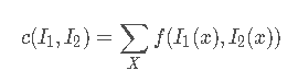
其中，函数f随着相关方法的变化而变化。上式取像素块中所有像素位置x的和。对于互相关矩阵，函数f(I1,I2)=I1I2，因此，c(I1,I2)=I1·I2，其中·表示向量乘法。c(I1,I2)的值越大，像素块I1和I2的相似度越高。

归一化的互相关矩阵是互相关矩阵的一种变形，可以定义为：

其中，n为像素块中像素的数目，μ1和μ2表示每个像素块中平均像素值强度，σ1和σ2分别表示每个像素块中的标准差。通过减去均值和除以标准差，该方法对图像亮度变化具有稳健性。

2.2例子

为获取图像像素块，并使用归一化的互相相关矩阵来比较它们，我们需要另外两个函数。
首先依旧是导入库，库报错说明你需要添加这个库：

from pylab import *
from PIL import Image
from numpy import *
import os

然后两个函数：

def get_descriptors(image, filtered_coords, wid=5):
    """对于每个返回的点，返回点周围2*wid+1个像素的值（假设选取点的min_distance > wid）"""

    desc = []
    for coords in filtered_coords:
        patch = image[coords[0]-wid:coords[0]+wid+1,
                coords[1]-wid:coords[1]+wid+1].flatten()
        desc.append(patch)

    return desc

def match(desc1, desc2, threshold=0.5):
    """对于第一幅图像中的每个角点描述子，使用归一化互相关，选取它在第二幅图像中的匹配角点"""
    
    n = len(desc1[0])
    
    # 点对的距离
    d = -ones((len(desc1), len(desc2)))
    for i in range(len(desc1)):
        for j in range(len(desc2)):
            d1 = (desc1[i] - mean(desc1[i])) / std(desc1[i])
            d2 = (desc2[j] - mean(desc2[j])) / std(desc2[j])
            ncc_value = sum(d1 *d2) / (n-1)
            if ncc_value > threshold:
                d[i,j] = ncc_value
    
    ndx = argsort(-d)
    matchscores = ndx[:,0]
    
    return matchscores

第一个函数的参数为奇数大小长度的方形灰度图像块，该图像块的中心为处理的像素点。该函数将图像块像素值压平成一个向量，然后添加到描述子列表中。第二个函数使用归一化的互相关矩阵，将每个描述子匹配到另一个图像中的最优候选点。由于数值较高的距离代表两个点能够更好的匹配，所以在排序之前，我们对距离取相反数。为了获得更稳定的匹配，我们从第二幅图像向第一幅图像匹配，然后过滤掉在两种方法中都不是最好的匹配。下面的函数可以实现该操作：

def match_twosided(desc1, desc2, threshold=0.5):
    """两边对称版本的match（）"""
    
    matches_12 = match(desc1, desc2, threshold)
    matches_21 = match(desc2, desc1, threshold)
    
    ndx_12 = where(matches_12 >= 0)[0]
    
    # 去除非对称的匹配
    for n in ndx_12:
        if matches_21[matches_12[n]] != n:
            matches_12[n] = -1
    
    return matches_12

这些匹配可以通过在两边分别绘制出图像，使用线段连接匹配的像素点来直观的可视化。下面代码可以实现匹配点的可视化。

def appendimages(im1, im2):
    """返回将两幅图像并排拼接成的一幅新图像"""
    
    # 选取具有最少行数的图像，然后填充足够的空行
    row1 = im1.shape[0]
    row2 = im2.shape[0]
    
    if row1 < row2:
        im1 = concatenate((im1,zeros((row2-row1,im1.shape[1]))), axis=0)
    elif row1 > row2:
        im2 = concatenate((im2,zeros((row1-row2,im2.shape[1]))), axis=0)
        
    # 如果这些情况都没有，那么他们的行数相同，不需要进行填充
    
    return concatenate((im1,im2), axis=1)

def plot_matches(im1, im2, locs1, locs2, matchscores, show_below=True):
    """显示一幅带有连接匹配之间连线的图片
        输入：im1，im2（数组图像），locs1，locs2（特征位置），matchscores（match的输出），
        show_below（如果图像应该显示再匹配下方）"""
    
    im3 = appendimages(im1,im2)
    if show_below:
        im3 = vstack((im3,im3))
        
    imshow(im3)
    
    cols1 = im1.shape[1]
    for i,m in enumerate(matchscores):
        if m > 0:
            plot([locs1[i][1],locs2[m][1]+cols1], [locs1[i][0], locs2[m][0]], 'c')
    axis('off')

具体实现函数：

im1 = array(Image.open('E:\学习\大三下\计算机视觉\第二章\jimei1.jpg').convert('L'))
im2 = array(Image.open('E:\学习\大三下\计算机视觉\第二章\jimei1.jpg').convert('L'))

wid = 5
harrisim = compute_harris_response(im1, 5)
filtered_coords1 = get_harris_points(harrisim, wid+1)
d1 = get_descriptors(im1, filtered_coords1, wid)

harrisim = compute_harris_response(im2, 5)
filtered_coords2 = get_harris_points(harrisim, wid + 1)
d2 = get_descriptors(im1, filtered_coords2, wid)

print('starting matching')
matches = match_twosided(d1,d2)

figure()
gray()
plot_matches(im1, im2, filtered_coords1, filtered_coords2, matches)
show()

结果截图：

为了看的更清楚，你可以画出匹配的子集。在上面的代码中，可以通过将数组matches替换成matches[:100]后者任意的子集来实现。

该算法的结果存在一些不正确匹配。这是因为，与现代的一些方法相比，图像像素块的互相关矩阵具有较弱的描述性。实际运用中，我们通常使用更稳健的方法来处理这些对应的匹配。这些描述符还有一个问题，他们不具有尺度不变性和旋转不变形，而算法中像素块的大小会影响对应匹配的结果。

近年来诞生了很多用来提高特征点检测和描述性能的方法。在下一小节，我们来学习其中最好的一种算法。

3 SIFT(尺度不变特征变换)

3.1介绍

SIFT，即尺度不变特征变换（Scale-invariant feature transform，SIFT），是用于图像处理领域的一种描述。这种描述具有尺度不变性，可在图像中检测出关键点，是一种局部特征描述子。 该方法于1999年由David Lowe 首先发表于计算机视觉国际会议（International Conference on Computer Vision，ICCV），2004年再次经David Lowe整理完善后发表于International journal of computer vision（IJCV）。截止2014年8月，该论文单篇被引次数达25000余次。
David Lowe提出的SIFT（Scale-Invariant Feature Transform，尺度不变特征变化）是过去十年中最成功的图像局部描述子之一。SIFT特征包括兴趣点检测器和描述子。SIFT描述子具有非常强的稳定性，这也是SIFT特征能够成功和流行的主要原因。SIFT特征对于尺度、旋转和亮度都具有不变性，因此，它可以用于三维视角和噪声的可靠匹配。

3.2兴趣点

SIFT特征使用高斯差分函数来定位兴趣点：

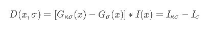
其中，Gσ是二维高斯核，Iσ是使用Gσ模糊的灰度图像，κ是决定相差尺度的常熟。兴趣点是在图像位置和尺度变换下D(x,σ)的最大值和最小值点。这些候选位置通过滤波去除不稳定点。基于一些准则，比如认为低对比度和位于边上的点不是兴趣点，我们可以去除一些候选兴趣点。

3.3描述子

上面讨论的兴趣点（关键点）位置描述子给出了兴趣点的位置和尺度信息。为了实现旋转不变性，基于每个点周围图像梯度的方向和大小，SIFT描述子又引入了参考方向。SIFT描述子使用主方向描述参考方向。主方向使用方向直方图（以大小为权重）来度量。

3.4检测兴趣点——例子

我们使用开源工具包VLFeat提供的二进制文件来计算图像的SIFT特征。
工具包VLFeat需要自己导入到环境，如何可以百度或者查看https://blog.csdn.net/grief_of_the_nazgul/article/details/49793809
导入库：

from pylab import *
from PIL import Image
from numpy import *
import os

将下面的函数添加到该文件：

def process_image(imagename, resultname, tmpname='tmp.pgm', params="--edge-thresh 10 --peak-thresh 5"):
    """处理一幅图像，然后将结果保存在文件中"""
    
    if imagename[-3:] != 'pgm':
        #创建一个pgm文件
        im = Image.open(imagename).convert('L')
        im.save(tmpname)
        imagename = tmpname
        
    cmmd= str("sift "+imagename+" --output="+resultname+" "+params)
    os.system(cmmd)
    print('processed',imagename,'to',resultname)

由于该二进制文件需要的图像格式为灰度.pgm，所以如果图像为其他各是，我们需要首先将其转换成.pgm格式文件。其中数据的每一行前4个数值依次表示兴趣点的坐标、尺度和方向角度，后面紧跟着的是对应描述符的128维向量。

下面函数用于从上面输出文件中，将特征读取到Numpy数组中的函数。

def read_features_from_file(filename):
    """读取特征值属性值，然后将其以矩阵形式返回"""
    
    f = loadtxt(filename)
    return f[:,:4],f[:,4:] # 特征位置，描述子

读取特征后，通过在图像上绘制出它们的位置，可以将其可视化。下面的函数可以实现这个功能

def plot_features(im, locs, circle=False):
    """显示带有特征的图像
        输入：im（数组图像），locs（每个特征的行、列、尺度和方向角度）"""

    def draw_circle(c,r):
        t = arange(0,1.01,.01)*2*pi
        x = r*cos(t) + c[0]
        y = r*sin(t) + c[1]
        plot(x,y,'b',linewidth=2)

    imshow(im)
    if circle:
        for p in locs:
            draw_circle(p[:2],p[2])
    else:
        plot(locs[:,0],locs[:,1],'ob')
    axis('off')
    return

我们通过下面的命令绘制SIFT特征位置的图像：

imname = 'E:/学习/大三下/计算机视觉/第二章/jimei1.jpg'
im1 = array(Image.open(imname).convert('L'))
process_image(imname,'jimei1.sift')
l1,d1 = read_features_from_file('E:/学习/大三下/计算机视觉/第二章/jimei1.sift')

figure()
gray()
plot_features(im1,l1,circle=True)
show()

结果截图：

3.5匹配描述子——例子

导入库：

from pylab import *
from PIL import Image
from numpy import *
import os

函数：

def process_image(imagename, resultname, params="--edge-thresh 10 --peak-thresh 5"):
    """处理一幅图像，然后将结果保存在文件中"""

    if imagename[-3:] != 'pgm':
        # 创建一个pgm文件
        im = Image.open(imagename).convert('L')
        im.save('tmp.pgm')
        imagename = 'tmp.pgm'

    cmmd = str("sift " + imagename + " --output=" + resultname + " " + params)
    os.system(cmmd)
    print('processed', imagename, 'to', resultname)


def read_features_from_file(filename):
    """读取特征值属性值，然后将其以矩阵形式返回"""

    f = loadtxt(filename)
    return f[:, :4], f[:, 4:]  # 特征位置，描述子

def plot_features(im, locs, circle=False):
    """显示带有特征的图像
        输入：im（数组图像），locs（每个特征的行、列、尺度和方向角度）"""

    def draw_circle(c,r):
        t = arange(0,1.01,.01)*2*pi
        x = r*cos(t) + c[0]
        y = r*sin(t) + c[1]
        plot(x,y,'b',linewidth=2)

    imshow(im)
    if circle:
        for p in locs:
            draw_circle(p[:2],p[2])
    else:
        plot(locs[:,0],locs[:,1],'ob')
    axis('off')
    return

def match(desc1, desc2):
    """对于第一幅图像的每个描述子，选取其在第二幅图像中的匹配
        输入：desc1（第一幅图像中的描述子），desc2（第二幅图像中的描述子）"""

    desc1 = array([d/linalg.norm(d) for d in desc1])
    desc2 = array([d/linalg.norm(d) for d in desc2])

    dist_ratio = 0.6
    desc1_size = desc1.shape

    matchscores = zeros((desc1_size[0],1), 'int')
    desc2t = desc2.T    #预先计算矩阵转置
    for i in range(desc1_size[0]):
        dotprods = dot(desc1[i,:], desc2t) #向量点乘
        dotprods = 0.9999*dotprods
        # 反余弦和反排序，返回第二幅图像中特征的索引
        index = argsort(arccos(dotprods))

        # 检查最近邻的角度是否小于dist_ratio乘以第二近邻的角度
        if arccos(dotprods)[index[0]] < dist_ratio * arccos(dotprods)[index[1]]:
            matchscores[i] = int(index[0])

    return matchscores

def match_twosided(desc1,decs2):
    """双向对称版本的match"""

    matches_12 = match(desc1, decs2)
    matches_21 = match(decs2, decs2)

    ndx_12 = matches_12.nonzero()[0]

    # 去除不对称匹配
    for n in ndx_12:

        if matches_21[int(matches_12[n])] != n:
            matches_12[n] = 0

    return matches_12

def appendimages(im1, im2):
    """返回将两幅图像并排拼接成的一幅新图像"""

    # 选取具有最少行数的图像，然后填充足够的空行
    row1 = im1.shape[0]
    row2 = im2.shape[0]

    if row1 < row2:
        im1 = concatenate((im1,zeros((row2-row1,im1.shape[1]))), axis=0)
    elif row1 > row2:
        im2 = concatenate((im2,zeros((row1-row2,im2.shape[1]))), axis=0)

    # 如果这些情况都没有，那么他们的行数相同，不需要进行填充

    return concatenate((im1,im2), axis=1)

def plot_matches(im1, im2, locs1, locs2, matchscores, show_below=True):
    """显示一幅带有连接匹配之间连线的图片
        输入：im1，im2（数组图像），locs1，locs2（特征位置），matchscores（match的输出），
        show_below（如果图像应该显示再匹配下方）"""

    im3 = appendimages(im1,im2)
    if show_below:
        im3 = vstack((im3,im3))

    imshow(im3)

    cols1 = im1.shape[1]
    for i in range(len(matchscores)):
        if matchscores[i] > 0:
            plot([locs1[i, 0], locs2[matchscores[i, 0], 0] + cols1], [locs1[i, 1], locs2[matchscores[i, 0], 1]], 'c')
    axis('off')

实现代码：

if __name__ == '__main__':
    im1f = r'E:/学习/大三下/计算机视觉/第二章/image/引桐楼1.jpg'
    im2f = r'E:/学习/大三下/计算机视觉/第二章/image/引桐楼2.jpg'
    im1 = array(Image.open(im1f))
    im2 = array(Image.open(im2f))

    process_image(im1f, 'out_sift_1.txt')
    l1, d1 = read_features_from_file('out_sift_1.txt')
    figure()
    gray()
    subplot(121)
    plot_features(im1, l1, circle=False)

    process_image(im2f, 'out_sift_2.txt')
    l2, d2 = read_features_from_file('out_sift_2.txt')
    subplot(122)
    plot_features(im2, l2, circle=False)

    matches = match_twosided(d1, d2)
    print('{} matches'.format(len(matches.nonzero()[0])))
    figure()
    gray()
    plot_matches(im1, im2, l1, l2, matches, show_below=True)
    show()

结果截图：

4 地理特征匹配

4.1需要安装PCV环境

在下载好了pcv的压缩包后，解压到当前文件夹就可以了

win+r ，输入cmd，打开命令行，先输入解压后的目录，在输入执行代码

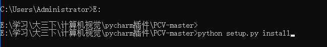
setup.py就是解压后目录里面有的

执行完后出现这个说明安装成功了：

4.2 测试图片

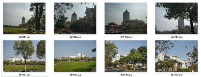
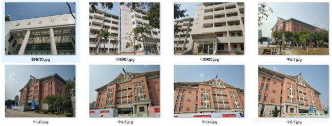
4.3实现代码

from pylab import *
from PIL import Image
from PCV.localdescriptors import sift
from PCV.tools import imtools
import pydot

if __name__ == '__main__':
    download_path = "E:/学习/大三下/计算机视觉/第二章/image"
    path = "E:/学习/大三下/计算机视觉/第二章/image"

    imlist = imtools.get_imlist(download_path)
    nbr_images = len(imlist)

    featlist = [imname[:-3] + 'sift' for imname in imlist]
    for i, imname in enumerate(imlist):
        sift.process_image(imname, featlist[i])

    matchscores = zeros((nbr_images, nbr_images))

    for i in range(nbr_images):
        for j in range(i, nbr_images):  # only compute upper triangle
            print('comparing ', imlist[i], imlist[j])
            l1, d1 = sift.read_features_from_file(featlist[i])
            l2, d2 = sift.read_features_from_file(featlist[j])
            matches = sift.match_twosided(d1, d2)
            nbr_matches = sum(matches > 0)
            print('number of matches = ', nbr_matches)
            matchscores[i, j] = nbr_matches

    # copy values
    for i in range(nbr_images):
        for j in range(i + 1, nbr_images):  # no need to copy diagonal
            matchscores[j, i] = matchscores[i, j]

    # 可视化

    threshold = 2  # min number of matches needed to create link

    g = pydot.Dot(graph_type='graph')  # don't want the default directed graph

    for i in range(nbr_images):
        for j in range(i + 1, nbr_images):
            if matchscores[i, j] > threshold:
                # first image in pair
                im = Image.open(imlist[i])
                im.thumbnail((100, 100))
                filename = path + str(i) + '.jpg'
                im.save(filename)  # need temporary files of the right size
                g.add_node(pydot.Node(str(i), fontcolor='transparent', shape='rectangle', image=filename))

                # second image in pair
                im = Image.open(imlist[j])
                im.thumbnail((100, 100))
                filename = path + str(j) + '.jpg'
                im.save(filename)  # need temporary files of the right size
                g.add_node(pydot.Node(str(j), fontcolor='transparent', shape='rectangle', image=filename))

                g.add_edge(pydot.Edge(str(i), str(j)))
    g.write_jpg('联系图.jpg')

结果图：

结果分析：

从结果看到测试用了16张图片，但是出来了是14张，其中有2张没有匹配出来。因为在上面代码的第42行设定了阈值theshhold=2，而有些图片特征点匹配的数量小于等于2，使得在可视化图片匹配的时候没有显示出来。
图书馆的5张图片只匹配了3张出来，应该也是应该角度变换过多的问题，导致特征点消失。