CS231n课后作业 | Assignment 3 Q4 | StyleTransfer-PyTorch 风格迁移

StyleTransfer-PyTorch

风格迁移

编写：BenVon

---

---

2018年的CS231n添加了StyleTransfer等新内容，同时添加了TensorFlow和PyTorch两种版本。目前网上主流的是TensorFlow的版本，在此更新一波PyTorch版本以供日后复习参考。

解答思路主要参考了 BigDataDigest 的 文章 ，汉化说明及TensorFlow代码可以看看这边。
我完成的PyTorch版本作业可以到 Github 上下载。

Style Transfer

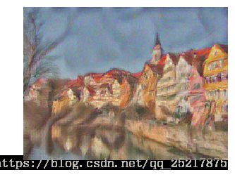
这个作业里我们将实现Image Style Transfer Using Convolutional Neural Networks” (Gatys et al., CVPR 2015)提到的风格转换技巧。

主要目的是准备两张图片，生成一张反映一张图的内容和另一张图的风格的新图。我们将通过计算深度网络中某一些特征空间中对应内容和风格的损失函数，并将梯度下降应用于图片像素本身。

我们使用SqueezeNet作为抽取特征的深度网络，这是一个在ImageNet上训练的小模型。你可以用任何网络，我们在这里选择SqueezeNet是因为它小而高效。

以下是一个你在本次作业最后可以完成的例子：

---

设置 Setup

import torch
import torch.nn as nn
import torchvision
import torchvision.transforms as T
import PIL

import numpy as np

from scipy.misc import imread
from collections import namedtuple
import matplotlib.pyplot as plt

from cs231n.image_utils import SQUEEZENET_MEAN, SQUEEZENET_STD
%matplotlib inline

我们准备了一些用于处理图片的帮助函数， 从这里 开始我们将处理真正的JPEGs数据，而非CIFAR-10数据。

def preprocess(img, size=512):
    transform = T.Compose([
        T.Resize(size),
        T.ToTensor(),
        T.Normalize(mean=SQUEEZENET_MEAN.tolist(),
                    std=SQUEEZENET_STD.tolist()),
        T.Lambda(lambda x: x[None]),
    ])
    return transform(img)

def deprocess(img):
    transform = T.Compose([
        T.Lambda(lambda x: x[0]),
        T.Normalize(mean=[0, 0, 0], std=[1.0 / s for s in SQUEEZENET_STD.tolist()]),
        T.Normalize(mean=[-m for m in SQUEEZENET_MEAN.tolist()], std=[1, 1, 1]),
        T.Lambda(rescale),
        T.ToPILImage(),
    ])
    return transform(img)

def rescale(x):
    low, high = x.min(), x.max()
    x_rescaled = (x - low) / (high - low)
    return x_rescaled

def rel_error(x,y):
    return np.max(np.abs(x - y) / (np.maximum(1e-8, np.abs(x) + np.abs(y))))

def features_from_img(imgpath, imgsize):
    img = preprocess(PIL.Image.open(imgpath), size=imgsize)
    img_var = img.type(dtype)
    return extract_features(img_var, cnn), img_var

# Older versions of scipy.misc.imresize yield different results
# from newer versions, so we check to make sure scipy is up to date.
def check_scipy():
    import scipy
    vnum = int(scipy.__version__.split('.')[1])
    major_vnum = int(scipy.__version__.split('.')[0])

    assert vnum >= 16 or major_vnum >= 1, "You must install SciPy >= 0.16.0 to complete this notebook."

check_scipy()

answers = dict(np.load('style-transfer-checks.npz'))

就像上一个assignment，我们需要设定dtype用于选择CPU或GPU。

dtype = torch.FloatTensor
# Uncomment out the following line if you're on a machine with a GPU set up for PyTorch!
#dtype = torch.cuda.FloatTensor 

# Load the pre-trained SqueezeNet model.
cnn = torchvision.models.squeezenet1_1(pretrained=True).features
cnn.type(dtype)

# We don't want to train the model any further, so we don't want PyTorch to waste computation 
# computing gradients on parameters we're never going to update.
for param in cnn.parameters():
    param.requires_grad = False

# We provide this helper code which takes an image, a model (cnn), and returns a list of
# feature maps, one per layer.
def extract_features(x, cnn):
    """
    Use the CNN to extract features from the input image x.

    Inputs:
    - x: A PyTorch Tensor of shape (N, C, H, W) holding a minibatch of images that
      will be fed to the CNN.
    - cnn: A PyTorch model that we will use to extract features.

    Returns:
    - features: A list of feature for the input images x extracted using the cnn model.
      features[i] is a PyTorch Tensor of shape (N, C_i, H_i, W_i); recall that features
      from different layers of the network may have different numbers of channels (C_i) and
      spatial dimensions (H_i, W_i).
    """
    features = []
    prev_feat = x
    for i, module in enumerate(cnn._modules.values()):
        next_feat = module(prev_feat)
        features.append(next_feat)
        prev_feat = next_feat
    return features

#please disregard warnings about initialization

---

计算损失 Computing Loss

我们将进行三个组成部分的损失函数的计算。损失函数 分为三个部分的和：内容损失+风格损失+整体多样性损失。

内容损失 Content Loss

我们可以通过将损失函数组合生成一张反映一张图的内容和另一张图的风格的图片。我们希望惩罚图片内容的偏移和风格的偏移。然后使用这个混合损失函数进行梯度下降，不是对模型的参数，而是对源图的像素值。

首先我们写出内容损失函数。内容损失评估了生成图像的特征图与源图像的特征图有多大区别。我们只关心网络其中一层的内容表达(假设是层 ℓ ℓ )，有特征图 Aℓ∈R1×Cℓ×Hℓ×Wℓ A ℓ ∈ R 1 × C ℓ × H ℓ × W ℓ 。 Cℓ C ℓ 是 ℓ ℓ 层滤波器/通道的数量， Hℓ H ℓ 和 Wℓ W ℓ 是高和宽。我们将对重构空间为一维的特征图进行运算。令 Fℓ∈RCℓ×Mℓ F ℓ ∈ R C ℓ × M ℓ 表示当前图像的特征图， Pℓ∈RCℓ×Mℓ P ℓ ∈ R C ℓ × M ℓ 表示内容源图的特征图，其中 Mℓ=Hℓ×Wℓ M ℓ = H ℓ × W ℓ 是每个特征图的元素数量。 Fℓ F ℓ 或 Pℓ P ℓ 的每一行表示了一个特定过滤器卷积了图片所有位置的向量化后的激励。最后，用 wc w c 表示内容损失部分在整体损失中的损失权值。
于是内容损失函数可以写为:

Lc=wc×∑i,j(Fℓij−Pℓij)2 L c = w c × ∑ i , j ( F i j ℓ − P i j ℓ ) 2

def content_loss(content_weight, content_current, content_original):
    """
    Compute the content loss for style transfer.

    Inputs:
    - content_weight: Scalar giving the weighting for the content loss.
    - content_current: features of the current image; this is a PyTorch Tensor of shape
      (1, C_l, H_l, W_l).
    - content_target: features of the content image, Tensor with shape (1, C_l, H_l, W_l).

    Returns:
    - scalar content loss
    """
    diff = content_current - content_original
    diff = diff*diff
    return content_weight * torch.sum(diff)

测试内容损失，误差应小于0.0001。

def content_loss_test(correct):
    content_image = 'styles/tubingen.jpg'
    image_size =  192
    content_layer = 3
    content_weight = 6e-2

    c_feats, content_img_var = features_from_img(content_image, image_size)

    bad_img = torch.zeros(*content_img_var.data.size()).type(dtype)
    feats = extract_features(bad_img, cnn)

    student_output = content_loss(content_weight, c_feats[content_layer], feats[content_layer]).cpu().data.numpy()
    error = rel_error(correct, student_output)
    print('Maximum error is {:.3f}'.format(error))

content_loss_test(answers['cl_out'])

Maximum error is 0.000

风格损失 Style Loss

现在我们可以来处理风格损失了。对于给定层 ℓ ℓ ，风格损失定义如下:
首先，计算一个用于表示每个滤波器的相关程度的Gram矩阵G，其中F与之前一样。Gram矩阵是一个协方差矩阵的近似，我们希望生成图片的激励状态与风格图片的激励状态相匹配，使(近似)协方差相匹配是其中的一种方法。你能用很多种方法完成，但Gram矩阵很好计算且在实践中有一个好结果，所以它很不错。
给定特征图 Fℓ F ℓ 形状为 (Cℓ,Mℓ) ( C ℓ , M ℓ ) ，Gram矩阵形状是 (Cℓ,Cℓ) ( C ℓ , C ℓ ) ， 它的项为:

Gℓij=∑kFℓikFℓjk G i j ℓ = ∑ k F i k ℓ F j k ℓ

假设 Gℓ G ℓ 是由当前图片的特征图算得的Gram矩阵， Aℓ A ℓ 是源图片的特征图算得的Gram矩阵， wℓ w ℓ 是可调权重，那么 ℓ ℓ 层的风格损失可以用两Gram矩阵的加权欧几里得距离表示:

Lℓs=wℓ∑i,j(Gℓij−Aℓij)2 L s ℓ = w ℓ ∑ i , j ( G i j ℓ − A i j ℓ ) 2

通常我们会计算一组层 L L 的风格损失而不是单独一层 ℓ ℓ ；完整风格损失是每一层风格损失的和:

Ls=∑ℓ∈LLℓs L s = ∑ ℓ ∈ L L s ℓ

从计算下面的Gram矩阵开始:

def gram_matrix(features, normalize=True):
    """
    Compute the Gram matrix from features.

    Inputs:
    - features: PyTorch Tensor of shape (N, C, H, W) giving features for
      a batch of N images.
    - normalize: optional, whether to normalize the Gram matrix
        If True, divide the Gram matrix by the number of neurons (H * W * C)

    Returns:
    - gram: PyTorch Tensor of shape (N, C, C) giving the
      (optionally normalized) Gram matrices for the N input images.
    """
    shape = features.size()
    features = features.view([shape[0],shape[1],-1])
    transpose_features = features.clone()
    # print(transpose_features.size())
    transpose_features = transpose_features.permute(0,2,1)
    # print(transpose_features.size())
    # print(features.size())
    result = torch.matmul(features, transpose_features)
    if normalize:
        result = result / (shape[0]*shape[1]*shape[2]*shape[3])
    return result

测试你的Gram矩阵代码，差值应该少于0.0001。

def gram_matrix_test(correct):
    style_image = 'styles/starry_night.jpg'
    style_size = 192
    feats, _ = features_from_img(style_image, style_size)
    student_output = gram_matrix(feats[5].clone()).cpu().data.numpy()
    error = rel_error(correct, student_output)
    print('Maximum error is {:.3f}'.format(error))

gram_matrix_test(answers['gm_out'])

Maximum error is 0.000

# Now put it together in the style_loss function...
def style_loss(feats, style_layers, style_targets, style_weights):
    """
    Computes the style loss at a set of layers.

    Inputs:
    - feats: list of the features at every layer of the current image, as produced by
      the extract_features function.
    - style_layers: List of layer indices into feats giving the layers to include in the
      style loss.
    - style_targets: List of the same length as style_layers, where style_targets[i] is
      a PyTorch Tensor giving the Gram matrix of the source style image computed at
      layer style_layers[i].
    - style_weights: List of the same length as style_layers, where style_weights[i]
      is a scalar giving the weight for the style loss at layer style_layers[i].

    Returns:
    - style_loss: A PyTorch Tensor holding a scalar giving the style loss.

    翻译一下：
    输入：
    - 特征： 目前图像每一层中的特征，来自于extract_features函数，即F`l
    - 风格层： 一系列涵盖了用于对计算style loss所使用features进行索引的索引变量
    - 风格目标： 一系列与style_layers长度相同，计算好源风格图Gram matrix的张量变量
    - 风格权值： 一系列与style_layers长度相同，用于分配权值的系数变量
    """
    # Hint: you can do this with one for loop over the style layers, and should
    # not be very much code (~5 lines). You will need to use your gram_matrix function.
    style_losses = 0
    for i in range(len(style_layers)):
        idx = style_layers[i]
        style_losses += content_loss(style_weights[i], 
                                     gram_matrix(feats[idx]), 
                                     style_targets[i]) 
    return style_losses

测试风格损失，差值应少于0.0001.

def style_loss_test(correct):
    content_image = 'styles/tubingen.jpg'
    style_image = 'styles/starry_night.jpg'
    image_size =  192
    style_size = 192
    style_layers = [1, 4, 6, 7]
    style_weights = [300000, 1000, 15, 3]

    c_feats, _ = features_from_img(content_image, image_size)    
    feats, _ = features_from_img(style_image, style_size)
    style_targets = []
    for idx in style_layers:
        style_targets.append(gram_matrix(feats[idx].clone()))

    student_output = style_loss(c_feats, style_layers, style_targets, style_weights).cpu().data.numpy()
    error = rel_error(correct, student_output)
    print('Error is {:.3f}'.format(error))


style_loss_test(answers['sl_out'])

Error is 0.000

整体方差正则化 Total-variation regularization

实际上对图像的平滑是有帮助的。我们可以通过在损失函数中添加一个用于处理像素值毛刺或者说整体偏差的项来实现。
你可以通过求每个像素与其周围相邻(水平或垂直)像素的差的平方和的累计值计算整体偏差。在这里我们求3个输入通道(RGB)的整体方差正则化的和，并用参数 wt w t 对其加权。

Ltv=wt×(∑c=13∑i=1H−1∑j=1W(xi+1,j,c−xi,j,c)2+∑c=13∑i=1H∑j=1W−1(xi,j+1,c−xi,j,c)2) L t v = w t × ( ∑ c = 1 3 ∑ i = 1 H − 1 ∑ j = 1 W ( x i + 1 , j , c − x i , j , c ) 2 + ∑ c = 1 3 ∑ i = 1 H ∑ j = 1 W − 1 ( x i , j + 1 , c − x i , j , c ) 2 )

在下一个Cell中，补充TV损失的定义。为了获得满分，你的实现不能有循环。

def tv_loss(img, tv_weight):
    """
    Compute total variation loss.

    Inputs:
    - img: PyTorch Variable of shape (1, 3, H, W) holding an input image.
    - tv_weight: Scalar giving the weight w_t to use for the TV loss.

    Returns:
    - loss: PyTorch Variable holding a scalar giving the total variation loss
      for img weighted by tv_weight.
    """
    # Your implementation should be vectorized and not require any loops!
    shape = img.size()
    row_cur = img[:, :, :-1, :]
    row_lat = img[:, :, 1:, :]
    col_cur = img[:, :, :, :-1]
    col_lat = img[:, :, :, 1:]
    row_result = row_lat - row_cur
    col_result = col_lat - col_cur
    row_result = row_result * row_result
    col_result = col_result * col_result    
    result = tv_weight * (torch.sum(row_result) + torch.sum(col_result))
    return result

测试你的TV损失实现，差值应小于0.0001。

def tv_loss_test(correct):
    content_image = 'styles/tubingen.jpg'
    image_size =  192
    tv_weight = 2e-2

    content_img = preprocess(PIL.Image.open(content_image), size=image_size)

    student_output = tv_loss(content_img, tv_weight).cpu().data.numpy()
    error = rel_error(correct, student_output)
    print('Error is {:.3f}'.format(error))

tv_loss_test(answers['tv_out'])

Error is 0.000

现在我们将所有东西串起来(下面这个函数你别动):

def style_transfer(content_image, style_image, image_size, style_size, content_layer, content_weight,
                   style_layers, style_weights, tv_weight, init_random = False):
    """
    Run style transfer!

    Inputs:
    - content_image: filename of content image
    - style_image: filename of style image
    - image_size: size of smallest image dimension (used for content loss and generated image)
    - style_size: size of smallest style image dimension
    - content_layer: layer to use for content loss
    - content_weight: weighting on content loss
    - style_layers: list of layers to use for style loss
    - style_weights: list of weights to use for each layer in style_layers
    - tv_weight: weight of total variation regularization term
    - init_random: initialize the starting image to uniform random noise
    """

    # Extract features for the content image
    content_img = preprocess(PIL.Image.open(content_image), size=image_size)
    feats = extract_features(content_img, cnn)
    content_target = feats[content_layer].clone()

    # Extract features for the style image
    style_img = preprocess(PIL.Image.open(style_image), size=style_size)
    feats = extract_features(style_img, cnn)
    style_targets = []
    for idx in style_layers:
        style_targets.append(gram_matrix(feats[idx].clone()))

    # Initialize output image to content image or nois
    if init_random:
        img = torch.Tensor(content_img.size()).uniform_(0, 1).type(dtype)
    else:
        img = content_img.clone().type(dtype)

    # We do want the gradient computed on our image!
    img.requires_grad_()

    # Set up optimization hyperparameters
    initial_lr = 3.0
    decayed_lr = 0.1
    decay_lr_at = 180

    # Note that we are optimizing the pixel values of the image by passing
    # in the img Torch tensor, whose requires_grad flag is set to True
    optimizer = torch.optim.Adam([img], lr=initial_lr)

    f, axarr = plt.subplots(1,2)
    axarr[0].axis('off')
    axarr[1].axis('off')
    axarr[0].set_title('Content Source Img.')
    axarr[1].set_title('Style Source Img.')
    axarr[0].imshow(deprocess(content_img.cpu()))
    axarr[1].imshow(deprocess(style_img.cpu()))
    plt.show()
    plt.figure()

    for t in range(200):
        if t < 190:
            img.data.clamp_(-1.5, 1.5)
        optimizer.zero_grad()

        feats = extract_features(img, cnn)

        # Compute loss
        c_loss = content_loss(content_weight, feats[content_layer], content_target)
        s_loss = style_loss(feats, style_layers, style_targets, style_weights)
        t_loss = tv_loss(img, tv_weight) 
        loss = c_loss + s_loss + t_loss

        loss.backward()

        # Perform gradient descents on our image values
        if t == decay_lr_at:
            optimizer = torch.optim.Adam([img], lr=decayed_lr)
        optimizer.step()

        if t % 100 == 0:
            print('Iteration {}'.format(t))
            plt.axis('off')
            plt.imshow(deprocess(img.data.cpu()))
            plt.show()
    print('Iteration {}'.format(t))
    plt.axis('off')
    plt.imshow(deprocess(img.data.cpu()))
    plt.show()

生成一些不错的图片 Generate some pretty pictures！

试试下面我们的三个不同参数组的style_transfer。确保运行所有三个Cell。你可以随意添加，但要确保你的作业中包含第三个参数组(星月夜)。

• content_image是内容图片的文件名
• style_image是风格图片的文件名
• image_size是内容图片最小图片维度的大小(用于内容损失和生成图片)
• style_size是风格图片最小图片维度的大小
• content_layer指定了内容损失计算层
• content_weight给出内容损失在损失函数中的权值。增加这个参数值会使得最后图片看起来更真实(与源图片内容更贴近)
• style_layers指定了一系列风格损失的计算层
• style_weight为style_layers中指定了一系列的每个layer的权值(每一个为整体风格损失做了一部分贡献)。我们通常给靠前的风格层更高的权值，因为他们描述了更局部/小规模的特征，对内容纹理比更大接受域的特征更重要。通常情况下，增加这些值会使得结果图片更不像源图片内容，而更像风格图片的表现。
• tv_weight指定了整体方差正则化在整体损失函数中的权值。增加这个值会使结果图片更平滑，但损失风格和内容的真实度。
  接下来三个Cells的代码(你不能更改超参数)，你可以随意复制粘贴各种参数来尝试看结果图片的变化。

# Composition VII + Tubingen
params1 = {
    'content_image' : 'styles/tubingen.jpg',
    'style_image' : 'styles/composition_vii.jpg',
    'image_size' : 192,
    'style_size' : 512,
    'content_layer' : 3,
    'content_weight' : 5e-2, 
    'style_layers' : (1, 4, 6, 7),
    'style_weights' : (20000, 500, 12, 1),
    'tv_weight' : 5e-2
}

style_transfer(**params1)

Iteration 0

Iteration 100

Iteration 199

# Scream + Tubingen
params2 = {
    'content_image':'styles/tubingen.jpg',
    'style_image':'styles/the_scream.jpg',
    'image_size':192,
    'style_size':224,
    'content_layer':3,
    'content_weight':3e-2,
    'style_layers':[1, 4, 6, 7],
    'style_weights':[200000, 800, 12, 1],
    'tv_weight':2e-2
}

style_transfer(**params2)

Iteration 0

Iteration 100

Iteration 199

# Starry Night + Tubingen
params3 = {
    'content_image' : 'styles/tubingen.jpg',
    'style_image' : 'styles/starry_night.jpg',
    'image_size' : 192,
    'style_size' : 192,
    'content_layer' : 3,
    'content_weight' : 6e-2,
    'style_layers' : [1, 4, 6, 7],
    'style_weights' : [300000, 1000, 15, 3],
    'tv_weight' : 2e-2
}

style_transfer(**params3)

Iteration 0

Iteration 100

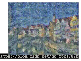
Iteration 199

特征反演 Feature Inversion

你完成的代码可以做另一件酷事儿。为了理解卷积神经网络学习识别的特征的类型，最近一篇文章1尝试通过图像的特征表达重构一张图片。我们可以通过在预训练网络中做图像梯度很容易实现这个想法，这也是我们上面实际上在做的(只不过永乐两个不同的特征表达)。
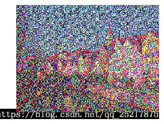
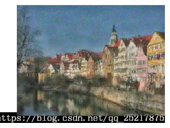
现在，如果你设置特征权值为0，并用随机噪点取代内容源图像进行初始化初始图像，你会通过图像的特征表达重构一张内容源图像。你将从完全的噪点开始，但你需要得到一个看起来与源图像相似的结果。
(类似的，你可以通过设置内容权值为0并初始化初始图像为随机噪点进行”纹理调理”，但是在此不做要求)
运行下面的Cell尝试特征反演。

# Feature Inversion -- Starry Night + Tubingen
params_inv = {
    'content_image' : 'styles/tubingen.jpg',
    'style_image' : 'styles/starry_night.jpg',
    'image_size' : 192,
    'style_size' : 192,
    'content_layer' : 3,
    'content_weight' : 6e-2,
    'style_layers' : [1, 4, 6, 7],
    'style_weights' : [0, 0, 0, 0], # we discard any contributions from style to the loss
    'tv_weight' : 2e-2,
    'init_random': True # we want to initialize our image to be random
}

style_transfer(**params_inv)

Iteration 0

Iteration 100

Iteration 199

---

1. Aravindh Mahendran, Andrea Vedaldi, “Understanding Deep Image Representations by Inverting them”, CVPR 2015 ↩