【吴恩达机器学习】Week5 编程作业ex4——神经网络学习
Neural Network
1. Visualizing the data
displayData.m
function [h, display_array] = displayData(X, example_width)
%DISPLAYDATA Display 2D data in a nice grid
%   [h, display_array] = DISPLAYDATA(X, example_width) displays 2D data
%   stored in X in a nice grid. It returns the figure handle h and the
%   displayed array if requested.

% Set example_width automatically if not passed in
if ~exist('example_width', 'var') || isempty(example_width)
	example_width = round(sqrt(size(X, 2)));
end

% Gray Image
colormap(gray);

% Compute rows, cols
[m n] = size(X);
example_height = (n / example_width);

% Compute number of items to display
display_rows = floor(sqrt(m));
display_cols = ceil(m / display_rows);

% Between images padding
pad = 1;

% Setup blank display
display_array = - ones(pad + display_rows * (example_height + pad), ...
                       pad + display_cols * (example_width + pad));

% Copy each example into a patch on the display array
curr_ex = 1;
for j = 1:display_rows
	for i = 1:display_cols
		if curr_ex > m,
			break;
		end
		% Copy the patch

		% Get the max value of the patch
		max_val = max(abs(X(curr_ex, :)));
		display_array(pad + (j - 1) * (example_height + pad) + (1:example_height), ...
		              pad + (i - 1) * (example_width + pad) + (1:example_width)) = ...
						reshape(X(curr_ex, :), example_height, example_width) / max_val;
		curr_ex = curr_ex + 1;
	end
	if curr_ex > m,
		break;
	end
end

% Display Image
h = imagesc(display_array, [-1 1]);

% Do not show axis
axis image off

drawnow;

end
ex4.m
%% Initialization
clear ; close all; clc

%% Setup the parameters you will use for this exercise
input_layer_size  = 400;  % 20x20 Input Images of Digits
hidden_layer_size = 25;   % 25 hidden units
num_labels = 10;          % 10 labels, from 1 to 10
                          % (note that we have mapped "0" to label 10)

%% =========== Part 1: Loading and Visualizing Data =============
%  We start the exercise by first loading and visualizing the dataset.
%  You will be working with a dataset that contains handwritten digits.
%

% Load Training Data
fprintf('Loading and Visualizing Data ...\n')

load('ex4data1.mat');
m = size(X, 1);

% Randomly select 100 data points to display
sel = randperm(size(X, 1));
sel = sel(1:100);

displayData(X(sel, :));

%fprintf('Program paused. Press enter to continue.\n');
%pause;
2. Model representation
%% ================ Part 2: Loading Parameters ================
% In this part of the exercise, we load some pre-initialized
% neural network parameters.

fprintf('\nLoading Saved Neural Network Parameters ...\n')

% Load the weights into variables Theta1 and Theta2
load('ex4weights.mat');

% Unroll parameters
nn_params = [Theta1(:) ; Theta2(:)];
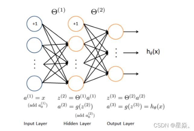
It has 3 layers – an input layer, a hidden layer and an output layer. Since the images are of size 20×20, this gives us 400 input layer units (not counting the extra bias unit which always outputs +1).
You have been provided with a set of network parameters (Θ(1),Θ(2)) already trained by us. These are stored in ex4weights.mat and will be loaded by ex4.m into Theta1 and Theta2. The parameters have dimensions that are sized for a neural network with 25 units in the second layer and 10 output units (corresponding to the 10 digit classes).
3. Feedforward and cost function
function [J grad] = nnCostFunction(nn_params, ...
                                   input_layer_size, ...
                                   hidden_layer_size, ...
                                   num_labels, ...
                                   X, y, lambda)
%NNCOSTFUNCTION Implements the neural network cost function for a two layer
%neural network which performs classification
%   [J grad] = NNCOSTFUNCTON(nn_params, hidden_layer_size, num_labels, ...
%   X, y, lambda) computes the cost and gradient of the neural network. The
%   parameters for the neural network are "unrolled" into the vector
%   nn_params and need to be converted back into the weight matrices.
%
%   The returned parameter grad should be a "unrolled" vector of the
%   partial derivatives of the neural network.
%

% Reshape nn_params back into the parameters Theta1 and Theta2, the weight matrices
% for our 2 layer neural network
Theta1 = reshape(nn_params(1:hidden_layer_size * (input_layer_size + 1)), ...
                 hidden_layer_size, (input_layer_size + 1));

Theta2 = reshape(nn_params((1 + (hidden_layer_size * (input_layer_size + 1))):end), ...
                 num_labels, (hidden_layer_size + 1));

% Setup some useful variables
m = size(X, 1);

% You need to return the following variables correctly
J = 0;
Theta1_grad = zeros(size(Theta1));
Theta2_grad = zeros(size(Theta2));


% ====================== YOUR CODE HERE ======================
% Instructions: You should complete the code by working through the
%               following parts.
%
% Part 1: Feedforward the neural network and return the cost in the
%         variable J. After implementing Part 1, you can verify that your
%         cost function computation is correct by verifying the cost
%         computed in ex4.m

% Training set (X,Y),数据预处理:将Y转换为目标向量形式
Y = zeros(m, size(Theta2, 1))
for i = 1 : size(Theta2, 1)
    Y(find(y == i), i) = 1;
end

% Set 各层的输入、输出:a、z
a1 = [ones(m, 1) X];             % input layer 5000x401
z2 = a1 * Theta1';                % hidden layer(in) 5000x25 where Theata 25x401
a2 = [ones(m, 1) sigmoid(z2)];   % hidden layer(out) 5000x26
z3 = a2 * Theta2';                % output layer(in) 5000x10 where Theta2 10x26
a3 = sigmoid(z3)                  % output result
h = a3                            % h_θ(x)


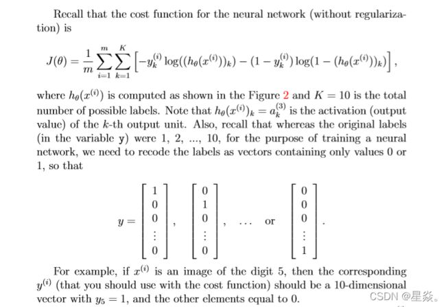
J = 1 / m * sum(sum(-Y .* log(h) - (1 - Y) .* log(1 - h)));
ex4.m
%% ================ Part 3: Compute Cost (Feedforward) ================
%  To the neural network, you should first start by implementing the
%  feedforward part of the neural network that returns the cost only. You
%  should complete the code in nnCostFunction.m to return cost. After
%  implementing the feedforward to compute the cost, you can verify that
%  your implementation is correct by verifying that you get the same cost
%  as us for the fixed debugging parameters.
%
%  We suggest implementing the feedforward cost *without* regularization
%  first so that it will be easier for you to debug. Later, in part 4, you
%  will get to implement the regularized cost.
%
fprintf('\nFeedforward Using Neural Network ...\n')

% Weight regularization parameter (we set this to 0 here).
lambda = 0;

J = nnCostFunction(nn_params, input_layer_size, hidden_layer_size, ...
                   num_labels, X, y, lambda);

fprintf(['Cost at parameters when lambda is equal to 0(loaded from ex4weights): %f '...
         '\n(this value should be about 0.287629)\n'], J);

%fprintf('\nProgram paused. Press enter to continue.\n');
%pause;
4. Regularized cost function
regTerm = lambda / (2 * m) * ...
            (sum(sum(Theta1(:, 2:size(Theta1, 2)).^2)) + ...
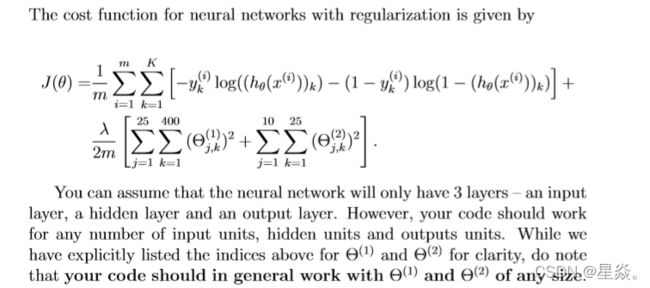
             sum(sum(Theta2(:, 2:size(Theta2, 2)).^2)));
J = J + regTerm;
ex4.m
%% ================ Part 3: Compute Cost (Feedforward) ================
%  To the neural network, you should first start by implementing the
%  feedforward part of the neural network that returns the cost only. You
%  should complete the code in nnCostFunction.m to return cost. After
%  implementing the feedforward to compute the cost, you can verify that
%  your implementation is correct by verifying that you get the same cost
%  as us for the fixed debugging parameters.
%
%  We suggest implementing the feedforward cost *without* regularization
%  first so that it will be easier for you to debug. Later, in part 4, you
%  will get to implement the regularized cost.
%
fprintf('\nFeedforward Using Neural Network ...\n')

% Weight regularization parameter (we set this to 0 here).
lambda = 1;

J = nnCostFunction(nn_params, input_layer_size, hidden_layer_size, ...
                   num_labels, X, y, lambda);


fprintf(['Cost at parameters when lambda is equal to 1(loaded from ex4weights): %f '...
         '\n(this value should be about 0.383770)\n'], J);

%fprintf('\nProgram paused. Press enter to continue.\n');
%pause;
Backpropagation
1. sigmoid gradient
function g = sigmoidGradient(z)
%SIGMOIDGRADIENT returns the gradient of the sigmoid function
%evaluated at z
%   g = SIGMOIDGRADIENT(z) computes the gradient of the sigmoid function
%   evaluated at z. This should work regardless if z is a matrix or a
%   vector. In particular, if z is a vector or matrix, you should return
%   the gradient for each element.

g = zeros(size(z));

% ====================== YOUR CODE HERE ======================
% Instructions: Compute the gradient of the sigmoid function evaluated at
%               each value of z (z can be a matrix, vector or scalar).

g = sigmoid(z) .* (1 - sigmoid(z));     % 既适用于矩阵,又适用于向量


% =============================================================


end
ex4.m
%% ================ Part 5: Sigmoid Gradient  ================
%  Before you start implementing the neural network, you will first
%  implement the gradient for the sigmoid function. You should complete the
%  code in the sigmoidGradient.m file.
%

fprintf('\nEvaluating sigmoid gradient...\n')

g = sigmoidGradient([-1 -0.5 0 0.5 1]);
fprintf('Sigmoid gradient evaluated at [-1 -0.5 0 0.5 1]:\n  ');
fprintf('%f ', g);
fprintf('\n\n');

%fprintf('Program paused. Press enter to continue.\n');
%pause;
2. Random initialization
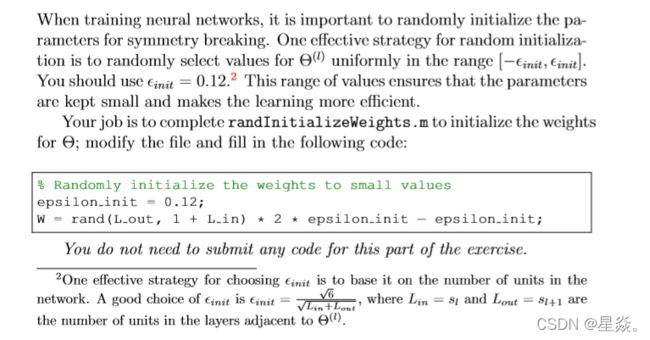
选取的 ϵ \epsilon ϵ 尽可能的小,一个有效的选取策略是以网络中的单元数量为基础,令 ϵ i n i t = 6 L i n + L o u t \epsilon_{init} = \frac{\sqrt{6}}{\sqrt{L_{in}+L_{out}}} ϵinit=Lin+Lout6,其中 L i n = s l L_{in} = s_l Lin=sl 和 L o u t = S l + 1 L_{out} = S_{l+1} Lout=Sl+1 是相邻 Θ ( l ) \Theta^{(l)} Θ(l) 的层中的单元数。
randInitializeWeights.m
function W = randInitializeWeights(L_in, L_out)
%RANDINITIALIZEWEIGHTS Randomly initialize the weights of a layer with L_in
%incoming connections and L_out outgoing connections
%   W = RANDINITIALIZEWEIGHTS(L_in, L_out) randomly initializes the weights
%   of a layer with L_in incoming connections and L_out outgoing
%   connections.
%
%   Note that W should be set to a matrix of size(L_out, 1 + L_in) as
%   the first column of W handles the "bias" terms
%

% You need to return the following variables correctly
W = zeros(L_out, 1 + L_in);

% ====================== YOUR CODE HERE ======================
% Instructions: Initialize W randomly so that we break the symmetry while
%               training the neural network.
%
% Note: The first column of W corresponds to the parameters for the bias unit
%

epsilon_init = 0.12;        %这个数字要小一点从而保证较高的学习效率
W = rando(L_out, 1 + L_in) * 2 * epsilon_init - epsillon_init;

% =========================================================================

end
3. Backpropagation
nnCostFunction.m
% Part 2: Implement the backpropagation algorithm to compute the gradients
%         Theta1_grad and Theta2_grad. You should return the partial derivatives of
%         the cost function with respect to Theta1 and Theta2 in Theta1_grad and
%         Theta2_grad, respectively. After implementing Part 2, you can check
%         that your implementation is correct by running checkNNGradients
%
%         Note: The vector y passed into the function is a vector of labels
%               containing values from 1..K. You need to map this vector into a
%               binary vector of 1's and 0's to be used with the neural network
%               cost function.
%
%         Hint: We recommend implementing backpropagation using a for-loop
%               over the training examples if you are implementing it for the
%               first time.

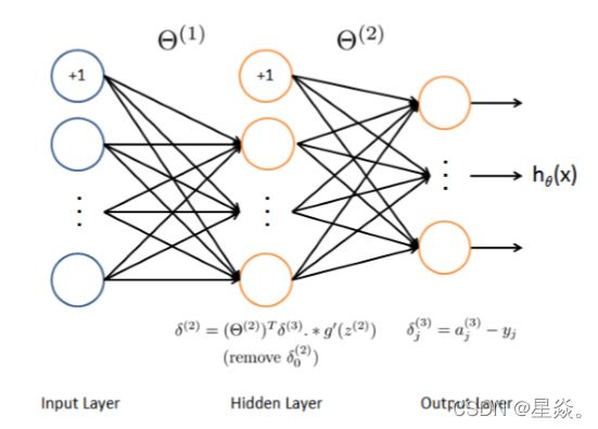
delta3 = a3 - Y;                        % 5000x10
delta2 = delta3 * Theta2;               % 5000x26
delta2 = delta2(:, 2:end);              % 5000x25
delta2 = delta2 .* sigmoidGradient(z2); % 5000x25

% Delta表示误差矩阵
Delta2 = zeros(size(Theta2));           % 10x26
Delta1 = zeros(size(Theta1));           % 25x401
Delta2 = Delta2 + delta3' * a2;         % 10x26     a2:5000x26
Delta1 = Delta1 + delta2' * a1;         % 25x401    a1:5000x401

Theta2_grad = 1 / m * Delta2;
Theta1_grad = 1 / m * Delta1;
ex4.m
%% =============== Part 7: Implement Backpropagation ===============
%  Once your cost matches up with ours, you should proceed to implement the
%  backpropagation algorithm for the neural network. You should add to the
%  code you've written in nnCostFunction.m to return the partial
%  derivatives of the parameters.
%
fprintf('\nChecking Backpropagation... \n');

%  Check gradients by running checkNNGradients
checkNNGradients;

%fprintf('\nProgram paused. Press enter to continue.\n');
%pause;
4. Gradient checking
function numgrad = computeNumericalGradient(J, theta)
%COMPUTENUMERICALGRADIENT Computes the gradient using "finite differences"
%and gives us a numerical estimate of the gradient.
%   numgrad = COMPUTENUMERICALGRADIENT(J, theta) computes the numerical
%   gradient of the function J around theta. Calling y = J(theta) should
%   return the function value at theta.

% Notes: The following code implements numerical gradient checking, and
%        returns the numerical gradient.It sets numgrad(i) to (a numerical
%        approximation of) the partial derivative of J with respect to the
%        i-th input argument, evaluated at theta. (i.e., numgrad(i) should
%        be the (approximately) the partial derivative of J with respect
%        to theta(i).)
%

numgrad = zeros(size(theta));
perturb = zeros(size(theta));
e = 1e-4;
for p = 1:numel(theta)
    % Set perturbation vector
    perturb(p) = e;
    loss1 = J(theta - perturb);
    loss2 = J(theta + perturb);
    % Compute Numerical Gradient
    numgrad(p) = (loss2 - loss1) / (2*e);
    perturb(p) = 0;
end

end
5. Regularized Neural Networks
% Part 3: Implement regularization with the cost function and gradients.
%
%         Hint: You can implement this around the code for
%               backpropagation. That is, you can compute the gradients for
%               the regularization separately and then add them to Theta1_grad
%               and Theta2_grad from Part 2.
%
Theta1_grad = 1 / m * Delta1 + lambda / m * Theta1;
Theta2_grad = 1 / m * Delta2 + lambda / m * Theta2;
Theta1_grad(:,1) = 1 / m * Delta1(:,1);
Theta2_grad(:,1) = 1 / m * Delta2(:,1);


% -------------------------------------------------------------
ex4.m
%% =============== Part 8: Implement Regularization ===============
%  Once your backpropagation implementation is correct, you should now
%  continue to implement the regularization with the cost and gradient.
%

fprintf('\nChecking Backpropagation (w/ Regularization) ... \n')

%  Check gradients by running checkNNGradients
lambda = 3;
checkNNGradients(lambda);

% Also output the costFunction debugging values
debug_J  = nnCostFunction(nn_params, input_layer_size, ...
                          hidden_layer_size, num_labels, X, y, lambda);

fprintf(['\n\nCost at (fixed) debugging parameters (w/ lambda = %f): %f ' ...
         '\n(for lambda = 3, this value should be about 0.576051)\n\n'], lambda, debug_J);

%fprintf('Program paused. Press enter to continue.\n');
%pause;
参考资料
吴恩达机器学习ex4-matlab版学习总结笔记-BP神经网络
吴恩达机器学习第五周编程作业ex4答案
全部作业代码
MLExercise_Ng
