线性回归(Linear Regression)
1. 数学描述
Y = θ 0 + θ 1 X 1 + ⋯ + θ i X i + ⋯ + θ n X n + ϵ Y=\theta_0+\theta_1 X_1+\cdots+\theta_iX_i+\cdots+\theta_nX_n+\epsilon Y=θ0+θ1X1+⋯+θiXi+⋯+θnXn+ϵ,其中:
- Y Y Y 是要预测的因变量(结果);
- X 1 , ⋯ , X n X_1,\cdots,X_n X1,⋯,Xn 是自变量(协变量)的特征;
- θ 0 \theta_0 θ0 是偏置, θ 1 , ⋯ , θ n \theta_1,\cdots,\theta_n θ1,⋯,θn 是权重系数,这些是需要学习和估计的;
- ϵ \epsilon ϵ 是偏差(随机误差),服从正态分布, ϵ ∼ N ( 0 , σ 2 ) \epsilon\sim N(0,\sigma^2) ϵ∼N(0,σ2),其中, σ 2 \sigma^2 σ2未知。
需要注意的是:模型强加了许多需要检查/证明的假设! Y Y Y 应该是连续的,不适合于分类/二进制因变量。 X i X_i Xi 既可以是连续的或离散的。
线性回归看起来是过于简单的,但这并不简单的意味着, Y Y Y 线性地依赖于 X i X_i Xi。但是线性回归是非常有用和重要的,它是非线性回归和许多先进回归模型的基本框架。
线性项指的是 θ i \theta_i θi ,而非 X i X_i Xi。如: Y = θ 0 + θ 1 X 1 + θ 2 e X 2 + ⋯ + θ i X i 3 + ⋯ + θ n X 2 X n + ϵ Y=\theta_0+\theta_1 X_1+\theta_2 e^{X_2}+\cdots+\theta_iX^3_i+\cdots+\theta_nX_2X_n+\epsilon Y=θ0+θ1X1+θ2eX2+⋯+θiXi3+⋯+θnX2Xn+ϵ,依然是一个线性回归模型。准确的说, X 1 , X 2 X_1,X_2 X1,X2 是协变量,而模型中的 X 1 , e X 2 , X i 3 , X 2 X n X_1,e^{X_2},X^3_i,X_2X_n X1,eX2,Xi3,X2Xn是预测因子或特征。
2 简单线性回归
若 Y = θ 0 + θ 1 X + ϵ Y=\theta_0+\theta_1 X+\epsilon Y=θ0+θ1X+ϵ,则在给定 X = x X=x X=x 时, Y Y Y 的条件均值是关于 x x x 的线性函数,
即: μ Y ∣ X = x = E ( Y ∣ X = x ) = θ 0 + θ 1 x \displaystyle \mu_{Y|X=x}=\mathrm E(Y|X=x)=\theta_0+\theta_1 x μY∣X=x=E(Y∣X=x)=θ0+θ1x.
若 θ 0 ^ , θ 1 ^ \hat{\theta_0},\hat{\theta_1} θ0^,θ1^ 分别是 θ 0 , θ 1 \theta_0,\theta_1 θ0,θ1的预估值,则有: μ ^ Y ∣ X = x = θ ^ 0 + θ ^ 1 x \displaystyle \hat\mu_{Y|X=x}=\hat\theta_0+\hat\theta_1 x μ^Y∣X=x=θ^0+θ^1x,这是 E ( Y ∣ X = x ) \mathrm E(Y|X=x) E(Y∣X=x) 的点估计。这是对所有 x x x 对应的平均因变量的估计。
同样的,使用 y ^ i = θ ^ 0 + θ ^ 1 x i \displaystyle \hat y_i=\hat\theta_0+\hat\theta_1 x_i y^i=θ^0+θ^1xi 作为当输入是 X = x i X=x_i X=xi 时的预测值, y i y_i yi 是真实值。令 e i = y i − y ^ i \displaystyle e_i=y_i-\hat y_i ei=yi−y^i 作为第 i i i 项的残差。
因此,定义 残差平方和(residual sum of squares ,RSS) 为: R S S ( θ 0 ^ , θ 1 ^ ) = ∑ i = 1 n e i 2 = ∑ i = 1 n ( y i − ( θ 0 ^ + θ 1 ^ x i ) ) 2 \displaystyle RSS(\hat{\theta_0},\hat{\theta_1})=\sum^n_{i=1}e^2_i=\sum^n_{i=1}(y_i-(\hat{\theta_0}+\hat{\theta_1}x_i))^2 RSS(θ0^,θ1^)=i=1∑nei2=i=1∑n(yi−(θ0^+θ1^xi))2,其中 { y i , x i , i = 1 , ⋯ , n } \{y_i,x_i,\;i=1,\cdots,n\} {yi,xi,i=1,⋯,n}是训练集。
能够使 R S S ( θ 0 ^ , θ 1 ^ ) RSS(\hat{\theta_0},\hat{\theta_1}) RSS(θ0^,θ1^) 最小的 θ 0 ^ , θ 1 ^ \hat{\theta_0},\hat{\theta_1} θ0^,θ1^ 就是最好的预测值,利用 最小二乘法(least squares method,LSM) 得到,可得: { θ 0 ^ = y ˉ − θ 1 ^ x ˉ , θ 1 ^ = ∑ ( x i − x ˉ ) ( y i − y ˉ ) ∑ ( x i − x ˉ ) 2 , \displaystyle \left\{ \begin{aligned} \hat{\theta_0}=\bar y-\hat{\theta_1}\bar x, \\ \hat{\theta_1}=\frac{\sum(x_i-\bar x)(y_i-\bar y)}{\sum(x_i-\bar x)^2}, \\ \end{aligned} \right. ⎩⎪⎨⎪⎧θ0^=yˉ−θ1^xˉ,θ1^=∑(xi−xˉ)2∑(xi−xˉ)(yi−yˉ),
其中, x ˉ , y ˉ \bar x, \bar y xˉ,yˉ 是训练集 x i , y i x_i, y_i xi,yi的均值。
3 一般情况的线性回归
3.1 常规数学计算
使用 最小均方(least mean squares,LMS) 进行一般化计算,其过程如下:

3.2 矩阵计算

3.3 概率阐述
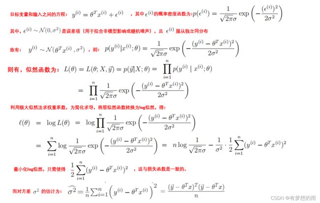
因为, E [ θ ^ ] = E [ ( X T X ) − 1 X T y ⃗ ] = E [ ( X T X ) − 1 X T ( θ T X + ϵ ) ] = θ + ( X T X ) − 1 X T E [ ϵ ] = θ \displaystyle\mathrm{E}[\hat{\theta}]=\mathrm{E}[\;(X^TX)^{-1}X^T\vec{y}\;]=\mathrm{E}[\;(X^TX)^{-1}X^T(\theta^TX+\epsilon)\;]=\theta+(X^TX)^{-1}X^T\mathrm{E}[\epsilon]=\theta E[θ^]=E[(XTX)−1XTy]=E[(XTX)−1XT(θTX+ϵ)]=θ+(XTX)−1XTE[ϵ]=θ
故, θ ^ \hat{\theta} θ^ 是 θ \theta θ 的无偏估计。
若 ϵ ( i ) ∼ N ( 0 , σ 2 ) \displaystyle \epsilon^{(i)}\sim\mathcal N(0,\sigma^2) ϵ(i)∼N(0,σ2),则有 θ ^ ∼ N ( θ , σ 2 ( X T X ) − 1 ) \displaystyle \hat\theta\sim\mathcal N(\theta,\sigma^2(X^TX)^{-1}) θ^∼N(θ,σ2(XTX)−1);
当 样本数量 n n n 足够大时,有 ( θ ^ σ ^ 2 ) ∼ N ( [ θ σ 2 ] , [ σ 2 ( X T X ) − 1 , 0 0 , 2 σ 4 n ] ) \displaystyle \left( \begin{array}{ccc}\hat{\theta} \\\hat\sigma^2\end{array} \right )\sim\mathcal N\left(\left[\begin{array}{ccc}{\theta} \\\sigma^2\end{array} \right ],\left[\begin{array}{ccc}\sigma^2(X^TX)^{-1}, &0 \\0,& \frac{2\sigma^4}{n}\end{array} \right ]\right ) (θ^σ^2)∼N([θσ2],[σ2(XTX)−1,0,0n2σ4])。
4. 正则化——岭回归(Ridge regression)
4.1 LMS求解的问题
利用最小二乘法对模型参数进行估计时,得到 θ ^ = ( X ′ X ) − 1 X ′ y ⃗ \hat\theta=(X'X)^{-1}X'\vec y θ^=(X′X)−1X′y;需要注意的是,该方法需要矩阵 X ′ X X'X X′X 的逆存在。
当 X ′ X X'X X′X 的逆不存在或者近似奇异时,有 E ∣ ∣ θ ^ − θ ∣ ∣ 2 = σ 2 ⋅ t r ( ( X ′ X ) − 1 ) \displaystyle\mathrm{E}||\hat{\theta}-\theta||^2=\sigma^2\cdot tr((X'X)^{-1}) E∣∣θ^−θ∣∣2=σ2⋅tr((X′X)−1)。其中, t r ( A ) tr(A) tr(A) 是矩阵 A A A 的迹,即 A A A 的对角线元素的和。
多重共线性问题(Multicollinearity issue):当 X X X 中至少有两列是强相关的,那么 X ′ X X'X X′X 几乎是奇异的。而当矩阵是接近奇异的,或矩阵规模很大时,结果往往是不准确的。
因此,对模型进行正则化是有必要的:
- 向学习问题的公式中添加一个额外的惩罚项以减少过拟合的风险;
- 对于学习算法的任何修正,目的都是减小 泛化误差,而非 训练误差。
添加正则项后,其公式化形式为: arg min f L ( f ( X ) , Y ) → arg min f L ( f ( x ) , Y ) + R ( f ) \displaystyle \argmin_fL(f(X),Y)\to\argmin_fL(f(x),Y)+R(f) fargminL(f(X),Y)→fargminL(f(x),Y)+R(f)
4.2 岭回归
当存在多重线性问题时,就需要在对参数 θ ^ \hat\theta θ^ 做估计时,需要对参数做出一些限制,如
∑ i = 0 n ( y ( i ) − θ 0 − θ 1 x 1 ( i ) − ⋯ − θ i x j ( i ) − ⋯ − θ p x p ( i ) ) 2 \displaystyle\sum^n_{i=0}(y^{(i)}-\theta_0-\theta_1 x^{(i)}_1-\cdots-\theta_ix^{(i)}_j-\cdots-\theta_px^{(i)}_p)^2 i=0∑n(y(i)−θ0−θ1x1(i)−⋯−θixj(i)−⋯−θpxp(i))2,需满足 ∑ j = 0 p θ j 2 < t \displaystyle\sum^p_{j=0}\theta_j^2
上述约束优化问题等价于: θ λ r i d g e = arg min θ ∑ i = 1 n ( y ( i ) − ∑ j = 0 p θ j x j ( i ) ) 2 + λ ∑ j = 1 p θ j 2 \displaystyle \theta^{ridge}_\lambda=\argmin_\theta\sum^n_{i=1}(y^{(i)}-\sum^p_{j=0}\theta_jx^{(i)}_j)^2+\lambda\sum^p_{j=1}\theta_j^2 θλridge=θargmini=1∑n(y(i)−j=0∑pθjxj(i))2+λj=1∑pθj2,其中, λ > 0 \lambda>0 λ>0 是缩放系数(shrinkage parameter)。
对上式的一些说明:
- 最小化带惩罚项的 RSS,其第二项控制参数的复杂度;
- 上式同时对误差项和模型复杂度进行优化;
- 注意到惩罚项不包括 θ 0 \theta_0 θ0;
- λ \lambda λ 用于控制惩罚项,需要提前选择。
对于大多数问题,为了数学表达上的便利,会对数据进行中心化归一处理,可使得 θ 0 = 0 \theta_0=0 θ0=0,则问题变为:
θ λ r i d g e = arg min θ ∑ i = 1 n ( y ( i ) − ∑ j = 1 p θ j x j ( i ) ) 2 + λ ∑ j = 1 p θ j 2 \displaystyle \theta^{ridge}_\lambda=\argmin_\theta\sum^n_{i=1}(y^{(i)}-\sum^p_{j=1}\theta_jx^{(i)}_j)^2+\lambda\sum^p_{j=1}\theta_j^2 θλridge=θargmini=1∑n(y(i)−j=1∑pθjxj(i))2+λj=1∑pθj2。
以矩阵化形式表述为: θ λ r i d g e = arg min θ ∣ ∣ y ⃗ − X θ ∣ ∣ 2 + λ θ T I p θ \displaystyle \theta^{ridge}_\lambda=\argmin_\theta ||\vec y-X\theta||^2+\lambda\theta^TI_p\theta θλridge=θargmin∣∣y−Xθ∣∣2+λθTIpθ,其中 X X X 不能是列向量, I p I_p Ip 是尺寸为 p p p 的单位阵。
- 可得, θ λ r i d g e = ( X T X + λ I p ) − 1 X T y ⃗ \displaystyle \theta^{ridge}_\lambda=(X^TX+\lambda I_p)^{-1}X^T\vec y θλridge=(XTX+λIp)−1XTy;
- 偏差:岭回归的 b i a s 2 bias^2 bias2 高于 最小二乘法;
- 方差:岭回归的方差小于最小二乘法;
- 当存在非零的 λ \lambda λ 时,岭回归的结果优于最小二乘法。
4.3 LASSO 回归
θ λ l a s s o = arg min θ ∑ i = 1 n ( y ( i ) − ∑ j = 0 p θ j x j ( i ) ) 2 + λ ∑ j = 1 p ∣ θ j ∣ \displaystyle \theta^{lasso}_\lambda=\argmin_\theta\sum^n_{i=1}(y^{(i)}-\sum^p_{j=0}\theta_jx^{(i)}_j)^2+\lambda\sum^p_{j=1}|\theta_j| θλlasso=θargmini=1∑n(y(i)−j=0∑pθjxj(i))2+λj=1∑p∣θj∣.
- LASSO 采用了另一种惩罚项,用系数的绝对值替代系数的平方;
- 当需要做变量选择时经常采用LASSO 回归,因为当 λ \lambda λ 足够大时,它会使得某些系数趋于变成 0;
- LASSO 具有更好的解释性,因为它可以生成稀疏解;
- 岭回归选择所有的特征做预测,这导致缺乏解释性,但是其预测误差更好。
4.4 贝叶斯视角下的正则化
贝叶斯理论: P ( θ ∣ D ) ∼ P ( D ∣ θ ) ⋅ P ( θ ) P(\theta|D)\sim P(D|\theta)\cdot P(\theta) P(θ∣D)∼P(D∣θ)⋅P(θ),其对应于 P o s t e r i o r ( 后 验 ) ∼ L i k e l i h o o d ( 似 然 ) ⋅ P r i o r ( 先 验 ) Posterior(后验)\sim Likelihood(似然)\cdot Prior(先验) Posterior(后验)∼Likelihood(似然)⋅Prior(先验);
- 若将 θ \theta θ 的先验视为给定方差,均值为 0 的高斯分布时,最大化后验,即可得到岭回归的形式;
- 若将先验视为 拉普拉斯分布(laplacian distributed),则可得到 LASSO回归。
4.5 弹性网络(elastic net)
即在岭回归和LASSO回归之间做一个折中:
θ ^ e n = arg min θ ∑ i = 1 n ( y ( i ) − ∑ j = 0 p θ j x j ( i ) ) 2 + λ ∑ j = 1 p ( α θ j 2 + ( 1 − α ) ∣ θ j ∣ ) \displaystyle \hat\theta_{en}=\argmin_\theta\sum^n_{i=1}(y^{(i)}-\sum^p_{j=0}\theta_jx^{(i)}_j)^2+\lambda\sum^p_{j=1}(\alpha\theta_j^2+(1-\alpha)|\theta_j|) θ^en=θargmini=1∑n(y(i)−j=0∑pθjxj(i))2+λj=1∑p(αθj2+(1−α)∣θj∣)
其中, λ ≥ 0 , 0 < α < 1 \lambda\ge0,0<\alpha<1 λ≥0,0<α<1。
弹性网络可以同 LASSO一样进行变量特征选择,同时像岭回归一样对相应的系数进行系数缩减。
5. Sklearn-Learning 中的线性回归模型
5.1标准线性回归
在机器学习库Sklearn-Learning 中,标准线性回归模型的接口如下:
sklearn.linear_model.LinearRegression(*, fit_intercept=True,
										normalize='deprecated',
										copy_X=True,
										n_jobs=None,
										positive=False)
其是一个拟合权重系数 w = ( w 1 , . . . , w p ) w = (w_1,... ,w_p) w=(w1,...,wp) 的线性模型,以最小化数据观测目标和线性近似预测目标之间的残差平方和。各项参数及其含义如下:
参数1:fit_intercept,bool类型,默认为 True,其含义为是否向模型中添加偏置项(及截断项)

参数2:normalize,bool类型, 默认为 False。
	当 fit_intercept=False 时该参数被忽略;
	如果 fit_intercept=True,回归变量 x 将在回归之前通过减去平均值除以 l2范数,即做归一化。

参数3:copy_X,bool类型, 默认为True。
	如果为真,x 将被复制; 否则,它会被覆盖。

参数4:n_jobs,int类型, default=None。
	设定用于计算的cpu核数量。如果 n_tragets > 1,而变量 X 又是稀疏的;或者如果 positive=True 时,会在大问题时提供加速。
	n_jobs = None 表示 核数量为1;
	n_jobs = -1 时,表示cpu中所有的核都参与工作。

参数5:positive,bool类型, default=False。
		当positive = True 时,强制系数为正。此选项仅支持稠密数组。
5.2 岭回归
在机器学习库Sklearn-Learning 中,岭回归模型的目标函数为:||y - Xw||^2_2 + alpha * ||w||^2_2,其函数接口如下:
sklearn.linear_model.Ridge(alpha=1.0, *,
							fit_intercept=True,
							normalize='deprecated',
							copy_X=True,
							max_iter=None,
							tol=0.001,
							solver='auto',
							positive=False,
							random_state=None)
其中,各项参数含义如下:
参数1: alpha, {float, ndarray of shape (n_targets,)}, default=1.0;
		当alpha是float时,用于控制正则项的强度,必须是大于0的实数;
		当alpha是ndarray时,则视为针对具体的目标系数进行惩罚,因此必须和目标系数数量相对于。

参数2:fit_intercept,bool类型,默认为 True,其含义为是否向模型中添加偏置项(及截断项)

参数3:normalize,bool类型, 默认为 False。
	当 fit_intercept=False 时该参数被忽略;
	如果 fit_intercept=True,回归变量 x 将在回归之前通过减去平均值除以 l2范数,即做归一化。

参数4:copy_X,bool类型, 默认为True。
	如果为真,x 将被复制; 否则,它会被覆盖。

参数5:max_iter,int类型, default=None,求解器的最大迭代次数;
		当求解器是'sparse_cg'或'lsqr'时,默认值由scipy.sparse.linalg决定;
		当求解器是'sag' 时,默认值是 1000;
		当求解器是 'lfbs'时,默认值是 15000;

参数6:tol,float类型, default=1e-3;
		解的精度;

参数7:solver,str类型,default='auto';求解器;
		'auto',基于输入的数据类型自动选择求解器;
		'svd',使用 x 的奇异值分解来计算岭回归系数。它是最稳定的求解器,特别是对于奇异矩阵来说,它比'cholesky'更稳定,但代价是速度更慢;
		'cholesky',使用标准的 scipy.linalg.solve 函数来获得一个封闭形式的解;
		'sparse_cg',使用共轭梯度求解器,如 scipy.sparse.linalg.cg。作为一种迭代算法,对于大规模数据(需要设置为 tol 和 max_iter) ,这种求解器比“ cholesky”更合适;
		'lsqr',‘ lsqr’使用专用的正则化最小二乘例程 scipy.sparse.linalg.lsqr,它是最快的,并使用了一个迭代过程;
		'sag',使用随机平均梯度下降法,'SAGA'使用改进后的无偏见版本,名为 SAGA。两种方法都使用了迭代过程,当 n 样本和 n 特征都很大时,它们通常比其他求解器更快。注意,'sag'和'saga'的快速收敛只有在大致相同规模的特征上才能得到保证;
		'lbfgs',使用在 scipy.optimize.minimize 中实现的 L-BFGS-B 算法,只有当positive为 True 时才能使用。
		注意:除了 'svd',所有的求解器都支持稀疏和稠密的数据;
			但是,只有当fit_intercept=True时,'lsqr','sag','sparse_cg','lbfgs'才能支持稀疏输入.

参数8:positive,bool类型, default=False。
		当positive = True 时,强制系数为正。此选项仅支持稠密数组。

参数9:random_state,int类型,  default=None;
		当求解器为 'sag'或'saga'时,该项用于控制打乱数据。
5.3 LASSO回归
在机器学习库Sklearn-Learning 中,LASSO回归模型的目标函数为:(1 / (2 * n_samples)) * ||y - Xw||^2_2 + alpha * ||w||_1,其函数接口如下:
sklearn.linear_model.Lasso(alpha=1.0, *,
							fit_intercept=True,
							normalize='deprecated',
							precompute=False,
							copy_X=True,
							max_iter=1000,
							tol=0.0001,
							warm_start=False,
							positive=False,
							random_state=None,
							selection='cyclic')
各项参数指标含义如下,与岭回归中有重复的在此不做重复描述:
参数4:precompute,bool 或 array-like of shape (n_features, n_features), default=False;
		是否使用预计算的 Gram 矩阵来加速计算;
		Gram 矩阵也可以作为参数传递;
		对于稀疏输入,此选项始终为 False 以保持稀疏性;

参数8:warm_start,bool类型,default=False;
		当warm_start=True 时,重用前一个调用的解决方案以适应初始化;
		否则,只需删除前一个解决方案;

参数11:selection,str类型,default='cyclic';
		如果selection='random',每次迭代都会更新一个随机系数;这(设置为“随机”)通常会导致明显加快收敛速度,特别是当 tol 高于1e-4时。
		如果selection='rcyclic',循环遍历。
5.4 弹性网络
在机器学习库Sklearn-Learning 中,弹性回归模型的目标函数为:1 / (2 * n_samples) * ||y - Xw||^2_2+ alpha * l1_ratio * ||w||_1+ 0.5 * alpha * (1 - l1_ratio) * ||w||^2_2,其函数接口如下:
sklearn.linear_model.ElasticNet(alpha=1.0, *,
								l1_ratio=0.5,
								fit_intercept=True,
								normalize='deprecated',
								precompute=False,
								max_iter=1000,
								copy_X=True,
								tol=0.0001,
								warm_start=False,
								positive=False,
								random_state=None,
								selection='cyclic')
各项参数指标含义如下,与LASSO回归中有重复的在此不做重复描述:
参数2:l1_ratio,float类型, default=0.5;
		用于控制 l1范数和 l2范数各自在惩罚项中的占比;