使用TensorFlow搭建几种经典的卷积神经网络：LeNet、AlexNet、VGGNet、InceptionNet、ResNet

1. LeNet1998

LeNet-5: Yann Lecun, Leon Bottou, Y. Bengio, Patrick Haffner. Gradient-Based Learning Applied to Document Recognition. Proceedings of the IEEE, 1998.

• 共享卷积核，减少网络参数

  LeNet-5虽然提出的时间比较早，但它是一个非常成功的神经网络模型。基于LeNet-5 的手写数字识别系统在20 世纪90 年代被美国很多银行使用，用来识别支票上面的手写数字。LeNet-5 的网络结构如下图所示。

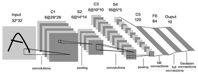
  LeNet-5由两层卷积层和三层全连接层组成，在Tensorflow框架下利用tf.Keras来构建LeNet5模型：

  与最初的LeNet5网络结构相比，这里做一点微调，输入图像尺寸为32 * 32 * 3，以适应cifar10数据集。模型中采用的激活函数有sigmoid和softmax，池化层均采用最大池化，以保留边缘特征。

#---------------
import tensorflow as tf
import os
import numpy as np
from matplotlib import pyplot as plt
from tensorflow.keras.layers import Conv2D, BatchNormalization, Activation, MaxPool2D, Dropout, Flatten, Dense
from tensorflow.keras import Model

np.set_printoptions(threshold=np.inf)
#---------------
cifar10 = tf.keras.datasets.cifar10
(x_train, y_train), (x_test, y_test) = cifar10.load_data()
x_train, x_test = x_train / 255.0, x_test / 255.0
#---------------
class LeNet5(Model):
    def __init__(self):
        super(LeNet5, self).__init__()
        self.c1 = Conv2D(filters=6, kernel_size=(5, 5),
                         activation='sigmoid')
        self.p1 = MaxPool2D(pool_size=(2, 2), strides=2)

        self.c2 = Conv2D(filters=16, kernel_size=(5, 5),
                         activation='sigmoid')
        self.p2 = MaxPool2D(pool_size=(2, 2), strides=2)

        self.flatten = Flatten()
        self.f1 = Dense(120, activation='sigmoid')
        self.f2 = Dense(84, activation='sigmoid')
        self.f3 = Dense(10, activation='softmax')

    def call(self, x):
        x = self.c1(x)
        x = self.p1(x)

        x = self.c2(x)
        x = self.p2(x)

        x = self.flatten(x)
        x = self.f1(x)
        x = self.f2(x)
        y = self.f3(x)
        return y

model = LeNet5()
#---------------
model.compile(optimizer='adam',
              loss=tf.keras.losses.SparseCategoricalCrossentropy(from_logits=False),
              metrics=['sparse_categorical_accuracy'])
#---------------
checkpoint_save_path = "./checkpoint/LeNet5.ckpt"
if os.path.exists(checkpoint_save_path + '.index'):
    print('-------------load the model-----------------')
    model.load_weights(checkpoint_save_path)

cp_callback = tf.keras.callbacks.ModelCheckpoint(filepath=checkpoint_save_path,
                                                 save_weights_only=True,
                                                 save_best_only=True)

history = model.fit(x_train, y_train, batch_size=32, epochs=5, validation_data=(x_test, y_test), validation_freq=1,
                    callbacks=[cp_callback])
#---------------
model.summary()
# print(model.trainable_variables)
file = open('./weights.txt', 'w')
for v in model.trainable_variables:
    file.write(str(v.name) + '\n')
    file.write(str(v.shape) + '\n')
    file.write(str(v.numpy()) + '\n')
file.close()
#------ show ------
# 显示训练集和验证集的acc和loss曲线
acc = history.history['sparse_categorical_accuracy']
val_acc = history.history['val_sparse_categorical_accuracy']
loss = history.history['loss']
val_loss = history.history['val_loss']

plt.subplot(1, 2, 1)
plt.plot(acc, label='Training Accuracy')
plt.plot(val_acc, label='Validation Accuracy')
plt.title('Training and Validation Accuracy')
plt.legend()

plt.subplot(1, 2, 2)
plt.plot(loss, label='Training Loss')
plt.plot(val_loss, label='Validation Loss')
plt.title('Training and Validation Loss')
plt.legend()
plt.show()

2. AlexNet2012

AlexNet: Alex Krizhevsky, Ilya Sutskever, Geoffrey E. Hinton. ImageNet Classification with Deep Convolutional Neural Networks. In NIPS, 2012.

• 激活函数使用ReLU，提升训练速度；
• Dropout防止过拟合，提升鲁棒性；
• 增加了一些训练上的技巧，包括数据增强、学习率衰减、权重衰减（L2正则化）等。

  AlexNet网络诞生于2012年，其ImageNet Top5错误率为16.4 %，可以说AlexNet的出现使得已经沉寂多年的深度学习领域开启了黄金时代。AlexNet由五层卷积、三层全连接组成，输入图像尺寸为$224\times 224\times 3$，输出为1000个类别的条件概率，网络规模远大于LeNet5，

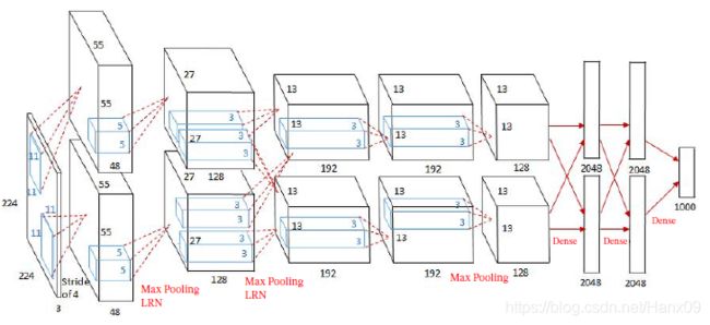
• 第一层卷积：卷积层使用两个大小为$11\times 11\times 11\times 3\times 48$的卷积核，步长$S=4$，零填充$P=3$，得到两个大小为$55\times 5\times 48$的特征映射组；汇聚层使用大小为$3\times 3$ 的最大汇聚操作，步长$S=2$，得到两个$27\times 27\times 48$ 的特征映射组；
• 第二层卷积：卷积层使用两个大小为$5\times 5\times 48\times 128$ 的卷积核，步长$S=1$，零填充$P=2$，得到两个大小为$27\times 27\times 128$ 的特征映射组；汇聚层使用大小为$3\times 3$ 的最大汇聚操作，步长$S=2$，得到两个大小为$13\times 13\times 128$ 的特征映射组；
• 第三层卷积：卷积层为两个路径的融合，使用一个大小为$3\times 3\times 256\times 384$的卷积核，步长$S=1$，零填充$P=1$，得到两个大小为$13\times 13\times 192$ 的特征映射组；
• 第四层卷积：卷积层使用两个大小为$3\times 3\times 192\times 192$ 的卷积核，步长$S=1$，零填充$P=1$，得到两个大小为$13\times 13\times 192$ 的特征映射组；
• 第五层卷积：卷积层使用两个大小为$3\times 3\times 192\times 128$ 的卷积核，步长$S=1$，零填充$P=1$，得到两个大小为$13\times 13\times 128$ 的特征映射组；汇聚层使用使用大小为$3\times 3$ 的最大汇聚操作，步长$S=2$，得到两个大小为$6\times 6\times 128$ 的特征映射组；
• 三个全连接层，神经元数量分别为4 096、4 096 和1 000。

  此外，AlexNet 还在前两个汇聚层之后进行了局部响应归一化（Local ResponseNormalization，LRN）以增强模型的泛化能力。

  在Tensorflow框架下利用Keras来搭建AlexNet模型，这里做了一些调整，将输入图像尺寸改为$32\times 32\times 3$以适应cifar10数据集，并且将原始的AlexNet模型中的$11\times 11$、$7\times 7$、$5\times 5$等大尺寸卷积核均替换成了$3\times 3$的小卷积核，

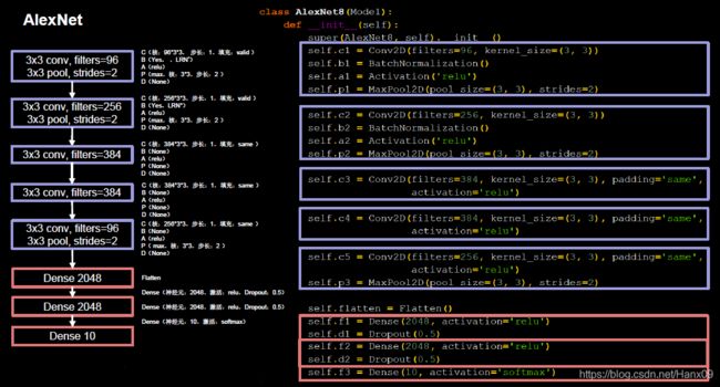
  与结构类似的LeNet5相比，AlexNet模型的参数量有了非常明显的提升，卷积运算的层数也更多了，这有利于更好地提取特征；Relu激活函数的使用加快了模型的训练速度；Dropout的使用提升了模型的鲁棒性，这些优势使得AlexNet的性能大大提升。

class AlexNet8(Model):
    def __init__(self):
        super(AlexNet8, self).__init__()
        self.c1 = Conv2D(filters=96, kernel_size=(3, 3))
        self.b1 = BatchNormalization()
        self.a1 = Activation('relu')
        self.p1 = MaxPool2D(pool_size=(3, 3), strides=2)

        self.c2 = Conv2D(filters=256, kernel_size=(3, 3))
        self.b2 = BatchNormalization()
        self.a2 = Activation('relu')
        self.p2 = MaxPool2D(pool_size=(3, 3), strides=2)

        self.c3 = Conv2D(filters=384, kernel_size=(3, 3), padding='same',
                         activation='relu')
                         
        self.c4 = Conv2D(filters=384, kernel_size=(3, 3), padding='same',
                         activation='relu')
                         
        self.c5 = Conv2D(filters=256, kernel_size=(3, 3), padding='same',
                         activation='relu')
        self.p3 = MaxPool2D(pool_size=(3, 3), strides=2)

        self.flatten = Flatten()
        self.f1 = Dense(2048, activation='relu')
        self.d1 = Dropout(0.5)
        self.f2 = Dense(2048, activation='relu')
        self.d2 = Dropout(0.5)
        self.f3 = Dense(10, activation='softmax')

    def call(self, x):
        x = self.c1(x)
        x = self.b1(x)
        x = self.a1(x)
        x = self.p1(x)

        x = self.c2(x)
        x = self.b2(x)
        x = self.a2(x)
        x = self.p2(x)

        x = self.c3(x)

        x = self.c4(x)

        x = self.c5(x)
        x = self.p3(x)

        x = self.flatten(x)
        x = self.f1(x)
        x = self.d1(x)
        x = self.f2(x)
        x = self.d2(x)
        y = self.f3(x)
        return y

model = AlexNet8()

3. VGGNet2014

VGG16: K. Simonyan, A. Zisserman. Very Deep Convolutional Networks for Large-Scale Image Recognition.In ICLR, 2015.

• 小卷积核减少参数的同时，提高识别准确率；
• 网络结构规整，适合并行加速。

  在AlexNet之后，另一个性能提升较大的网络是诞生于2014年的VGGNet，其ImageNet Top5错误率减小到了7.3 %。VGGNet网络的最大改进是在网络的深度上，由AlexNet的8层增加到了16层和19层，更深的网络意味着更强的表达能力，这得益于强大的运算能力支持。VGGNet的另一个显著特点是仅使用了单一尺寸的$3\times 3$卷积核，事实上，$3\times 3$的小卷积核在很多卷积网络中都被大量使用，这是由于在感受野相同的情况下，小卷积核堆积的效果要优于大卷积核，同时参数量也更少。
  VGGNet16和VGGNet19并没有本质上的区别，只是网络深度不同，前者16层（13层卷积、3层全连接），后者19层（16层卷积、3层全连接）。VGGNet16的网络结构如下图所示：

  越靠后，特征图尺寸越小，通过增加卷积核的个数，增加了特征图深度，保持了信息的承载能力。在Tensorflow框架下利用Keras来实现VGG16网络，为适应cifar10数据集，将输入图像尺寸由$224\times 244\times 3$调整为$32\times 32\times 3$，

class VGG16(Model):
    def __init__(self):
        super(VGG16, self).__init__()
        self.c1 = Conv2D(filters=64, kernel_size=(3, 3), padding='same')  # 卷积层1
        self.b1 = BatchNormalization()  # BN层1
        self.a1 = Activation('relu')  # 激活层1
        self.c2 = Conv2D(filters=64, kernel_size=(3, 3), padding='same', )
        self.b2 = BatchNormalization()  # BN层1
        self.a2 = Activation('relu')  # 激活层1
        self.p1 = MaxPool2D(pool_size=(2, 2), strides=2, padding='same')
        self.d1 = Dropout(0.2)  # dropout层

        self.c3 = Conv2D(filters=128, kernel_size=(3, 3), padding='same')
        self.b3 = BatchNormalization()  # BN层1
        self.a3 = Activation('relu')  # 激活层1
        self.c4 = Conv2D(filters=128, kernel_size=(3, 3), padding='same')
        self.b4 = BatchNormalization()  # BN层1
        self.a4 = Activation('relu')  # 激活层1
        self.p2 = MaxPool2D(pool_size=(2, 2), strides=2, padding='same')
        self.d2 = Dropout(0.2)  # dropout层

        self.c5 = Conv2D(filters=256, kernel_size=(3, 3), padding='same')
        self.b5 = BatchNormalization()  # BN层1
        self.a5 = Activation('relu')  # 激活层1
        self.c6 = Conv2D(filters=256, kernel_size=(3, 3), padding='same')
        self.b6 = BatchNormalization()  # BN层1
        self.a6 = Activation('relu')  # 激活层1
        self.c7 = Conv2D(filters=256, kernel_size=(3, 3), padding='same')
        self.b7 = BatchNormalization()
        self.a7 = Activation('relu')
        self.p3 = MaxPool2D(pool_size=(2, 2), strides=2, padding='same')
        self.d3 = Dropout(0.2)

        self.c8 = Conv2D(filters=512, kernel_size=(3, 3), padding='same')
        self.b8 = BatchNormalization()  # BN层1
        self.a8 = Activation('relu')  # 激活层1
        self.c9 = Conv2D(filters=512, kernel_size=(3, 3), padding='same')
        self.b9 = BatchNormalization()  # BN层1
        self.a9 = Activation('relu')  # 激活层1
        self.c10 = Conv2D(filters=512, kernel_size=(3, 3), padding='same')
        self.b10 = BatchNormalization()
        self.a10 = Activation('relu')
        self.p4 = MaxPool2D(pool_size=(2, 2), strides=2, padding='same')
        self.d4 = Dropout(0.2)

        self.c11 = Conv2D(filters=512, kernel_size=(3, 3), padding='same')
        self.b11 = BatchNormalization()  # BN层1
        self.a11 = Activation('relu')  # 激活层1
        self.c12 = Conv2D(filters=512, kernel_size=(3, 3), padding='same')
        self.b12 = BatchNormalization()  # BN层1
        self.a12 = Activation('relu')  # 激活层1
        self.c13 = Conv2D(filters=512, kernel_size=(3, 3), padding='same')
        self.b13 = BatchNormalization()
        self.a13 = Activation('relu')
        self.p5 = MaxPool2D(pool_size=(2, 2), strides=2, padding='same')
        self.d5 = Dropout(0.2)

        self.flatten = Flatten()
        self.f1 = Dense(512, activation='relu')
        self.d6 = Dropout(0.2)
        self.f2 = Dense(512, activation='relu')
        self.d7 = Dropout(0.2)
        self.f3 = Dense(10, activation='softmax')

    def call(self, x):
        x = self.c1(x)
        x = self.b1(x)
        x = self.a1(x)
        x = self.c2(x)
        x = self.b2(x)
        x = self.a2(x)
        x = self.p1(x)
        x = self.d1(x)

        x = self.c3(x)
        x = self.b3(x)
        x = self.a3(x)
        x = self.c4(x)
        x = self.b4(x)
        x = self.a4(x)
        x = self.p2(x)
        x = self.d2(x)

        x = self.c5(x)
        x = self.b5(x)
        x = self.a5(x)
        x = self.c6(x)
        x = self.b6(x)
        x = self.a6(x)
        x = self.c7(x)
        x = self.b7(x)
        x = self.a7(x)
        x = self.p3(x)
        x = self.d3(x)

        x = self.c8(x)
        x = self.b8(x)
        x = self.a8(x)
        x = self.c9(x)
        x = self.b9(x)
        x = self.a9(x)
        x = self.c10(x)
        x = self.b10(x)
        x = self.a10(x)
        x = self.p4(x)
        x = self.d4(x)

        x = self.c11(x)
        x = self.b11(x)
        x = self.a11(x)
        x = self.c12(x)
        x = self.b12(x)
        x = self.a12(x)
        x = self.c13(x)
        x = self.b13(x)
        x = self.a13(x)
        x = self.p5(x)
        x = self.d5(x)

        x = self.flatten(x)
        x = self.f1(x)
        x = self.d6(x)
        x = self.f2(x)
        x = self.d7(x)
        y = self.f3(x)
        return y

model = VGG16()

4. InceptionNet2014

Inception-v1: Szegedy C, Liu W, Jia Y, et al. Going Deeper with Convolutions. In CVPR, 2015.

• 引入Inception结构块，一层网络内使用多个不同尺寸的卷积核，提升了模型感知力（通过padding实现输出特征面积一致）；
• 使用$1\times 1$卷积核，改变输出特征channel数；
• 通过设定小于输入特征图深度的$1\times 1$卷积核个数，减少了输出特征图深度，起到了降维的作用，减少了参数量和计算量；
• 使用批标准化，缓解了梯度消失；
• GoogLeNet/Inception v1、Inception v2、v3、v4都是基于Inception结构块搭建的网络。

  InceptionNet即GoogLeNet，诞生于2015年，旨在通过增加网络的宽度来提升网络的能力，与VGGNet通过卷积层堆叠的方式（纵向）相比，是一个不同的方向（横向）。在Inception 网络中，一个卷积层包含多个不同大小的卷积操作，称为InceptionNet的基本单元，Inception 网络是由有多个Inception基本单元和少量的汇聚层堆叠而成。

InceptionNet基本单元

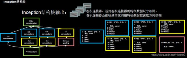
  InceptionNet最原始的基本单元结构如下图所示，

  可以看出InceptionNet最初的设计思想是，通过不同尺寸卷积层和池化层的横向组合（卷积、池化后的尺寸相同，通道可以相加）来拓宽网络深度，可以增加网络对尺寸的适应性。但是这样也带来一个问题，所有的卷积核都会在上一层的输出上直接做卷积运算，会导致参数量和计算量过大（尤其是对于5 * 5的卷积核来说）。因此，InceptionNet在$3\times 3$、$5\times 5$的卷积运算前、$3\times 3$的最大池化后均加入了$1\times 1$的卷积层来减少特征映射的深度，形成了下图中的结构，这样可以降低特征的厚度，一定程度上避免参数量过大的问题，如果输入特征映射之间存在冗余信息，$1\times 1$的卷积相当于先进行一次特征抽取。

---

$1\times 1$的卷积运算如何降低特征厚度：

  下面以$5\times 5$的卷积运算为例说明这个问题。

• 假设网络上一层的输出为$100\times 100\times 128（Height\times Width\times Channel）$，通过$32\times 5\times 5$（32个大小为$5\times 5$的卷积核）的卷积层（步长为1、全零填充）后，输出为$100\times 100\times 32$，卷积层的参数量为$32\times 5\times 5\times 128=102400$；
• 如果先通过$32\times 1\times 1$的卷积层（输出为$100\times 100\times 32$），再通过$32\times 5\times 5$的卷积层，输出仍为$100\times 100\times 32$，但卷积层的参数量变为$32\times 1\times 1\times 128+32\times 5\times 5\times 32=29696$，仅为原参数量的30 %左右，这就是小卷积核的降维作用。

---

  InceptionNet的基本单元中，卷积部分是比较统一的C、B、A典型结构，即卷积$\to$BN$\to$激活，激活均采用Relu激活函数，同时包含最大池化操作。在Tensorflow框架下利用Keras构建InceptionNet模型时，可以将C、B、A结构封装在一起，定义成一个新的ConvBNRelu类，以减少代码量，同时更便于阅读。

#ch：特征图的通道数，即卷积核个数
#kernelsz：卷积核尺寸
#strides：卷积步长
#padding：是否进行全零填充
class ConvBNRelu(Model):
    def __init__(self, ch, kernelsz=3, strides=1, padding='same'):
        super(ConvBNRelu, self).__init__()
        self.model = tf.keras.models.Sequential([
            Conv2D(ch, kernelsz, strides=strides, padding=padding),
            BatchNormalization(),
            Activation('relu')
        ])

    def call(self, x):
        x = self.model(x, training=False) #在training=False时，BN通过整个训练集计算均值、方差去做批归一化，training=True时，通过当前batch的均值、方差去做批归一化。推理时 training=False效果好
        return x

  完成了这一步后，就可以开始构建InceptionNet的基本单元了，同样利用class定义的方式，定义一个新的InceptionBlk类。

class InceptionBlk(Model):
    def __init__(self, ch, strides=1):
        super(InceptionBlk, self).__init__()
        self.ch = ch
        self.strides = strides
        self.c1 = ConvBNRelu(ch, kernelsz=1, strides=strides)
        self.c2_1 = ConvBNRelu(ch, kernelsz=1, strides=strides)
        self.c2_2 = ConvBNRelu(ch, kernelsz=3, strides=1)
        self.c3_1 = ConvBNRelu(ch, kernelsz=1, strides=strides)
        self.c3_2 = ConvBNRelu(ch, kernelsz=5, strides=1)
        self.p4_1 = MaxPool2D(3, strides=1, padding='same')
        self.c4_2 = ConvBNRelu(ch, kernelsz=1, strides=strides)

    def call(self, x):
        x1 = self.c1(x)
        x2_1 = self.c2_1(x)
        x2_2 = self.c2_2(x2_1)
        x3_1 = self.c3_1(x)
        x3_2 = self.c3_2(x3_1)
        x4_1 = self.p4_1(x)
        x4_2 = self.c4_2(x4_1)
        # concat along axis=channel
        x = tf.concat([x1, x2_2, x3_2, x4_2], axis=3)
        return x

其中，tf.concat函数将四个输出连接在一起

InceptionNet

  InceptionNet网络的主体就是由其基本单元构成的，其模型结构如下图所示。

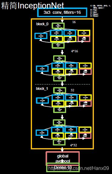
  图中橙色框内即为InceptionNet的基本单元，利用之前定义好的InceptionBlk类堆叠而成，模型的实现代码如下。

  参数num_layers代表InceptionNet的Block数，每个Block由两个基本单元构成，每经过一个Block，特征图尺寸变为1/2，通道数变为2倍；num_classes代表分类数，对于cifar10数据集来说即为10；init_ch代表初始通道数，也即InceptionNet基本单元的初始卷积核个数。InceptionNet网络不再像VGGNet一样有三层全连接层（全连接层的参数量占VGGNet总参数量的90 %），而是采用“全局平均池化+全连接层”的方式，这减少了大量的参数。

  全局平均池化在tf.keras中用GlobalAveragePooling2D函数实现，相比于平均池化（在特征图上以窗口的形式滑动，取窗口内的平均值为采样值），全局平均池化不再以窗口滑动的形式取均值，而是直接针对特征图取平均值，即每个特征图输出一个值。通过这种方式，每个特征图都与分类概率直接联系起来，这替代了全连接层的功能，并且不产生额外的训练参数，减小了过拟合的可能，但需要注意的是，使用全局平均池化会导致网络收敛的速度变慢。

  总体来看，InceptionNet采取了多尺寸卷积再聚合的方式拓宽网络结构，并通过$1\times 1$的卷积运算来减小参数量，取得了比较好的效果，与同年诞生的VGGNet相比，提供了卷积神经网络构建的另一种思路。但InceptionNet的问题是，当网络深度不断增加时，训练会十分困难，甚至无法收敛（这一点被ResNet很好地解决了）。

---

  GoogLeNet 由9 个Inception v1 模块和5 个汇聚层以及其他一些卷积层和全连接层构成，总共为22 层网络：（清晰GoogleNet图）

---

5. ResNet2015

ResNet: Kaiming He, Xiangyu Zhang, Shaoqing Ren. Deep Residual Learning for Image Recognition. In CPVR, 2016.

• 层间残差跳连，引入前方信息，减少梯度消失，使网络层数变身成为可能。

  ResNet即深度残差网络，由何恺明及其团队提出，是深度学习领域又一具有开创性的工作，通过对残差结构的运用，ResNet使得训练数百层的网络成为了可能，从而具有非常强大的表征能力，其网络结构如下图所示。

  ResNet的核心是残差结构，如下图所示，

  这里的相加与InceptionNet中的相加是有本质区别的：

• Inception块中的“+”是沿深度方向叠加（千层蛋糕层数叠加）；
• ResNet块中的“+”是特征图对应元素值相加（矩阵值相加）。

  在残差结构中，ResNet不再让下一层直接拟合我们想得到的底层映射，而是令其对一种残差映射进行拟合。假设在一个深度网络中，期望一个用非线性单元（一层或多层的卷积层）$f(x)$去逼近目标函数$h(x)$，如果将目标函数拆分为两部分：恒等函数$x$和残差函数$h(x)-x$，
$$h(x)=x+(h(x)-x)$$

根据通用近似定理，一个由神经网络构成的非线性单元有足够的能力来近似逼近原始目标函数或残差函数，但实际中后者更容易学习：不妨考虑极限情况，如果一个恒等映射是最优的，那么将残差向零逼近显然会比利用大量非线性层直接进行拟合更容易。因此，原来的优化问题可以转换为：让非线性单元$f(x)$去近似残差函数$h(x)-x$，并用$f(x)+x$去逼近$h(x)$。

  ResNet引入残差结构最主要的目的是解决网络层数不断加深时导致的梯度消失问题，从之前介绍的4种CNN经典网络结构我们也可以看出，网络层数的发展趋势是不断加深的。这是由于深度网络本身集成了低层/中层/高层特征和分类器，以多层首尾相连的方式存在，所以可以通过增加堆叠的层数（深度）来丰富特征的层次，以取得更好的效果。

  但如果只是简单地堆叠更多层数，就会导致梯度消失（爆炸）问题，它从根源上导致了函数无法收敛。然而，通过标准初始化（normalized initialization）以及中间标准化层（intermediate normalization layer），已经可以较好地解决这个问题了，这使得深度为数十层的网络在反向传播过程中，可以通过随机梯度下降（SGD）的方式开始收敛。

  但是，当深度更深的网络也可以开始收敛时，网络退化的问题就显露了出来：随着网络深度的增加，准确率先是达到瓶颈（这是很常见的），然后便开始迅速下降。需要注意的是，这种退化并不是由过拟合引起的。对于一个深度比较合适的网络来说，继续增加层数反而会导致训练错误率的提升，

  ResNet解决的正是这个问题，其核心思路为：对一个准确率达到饱和的浅层网络，在它后面加几个恒等映射层（即y = x，输出等于输入），增加网络深度的同时不增加误差。这使得神经网络的层数可以超越之前的约束，提高准确率。

  使用tf.keras来实现这种残差结构，定义一个ResnetBlock类：卷积操作仍然采用典型的C、B、A结构，激活采用Relu函数；为了保证F(x)和x可以顺利相加，二者的维度必须相同，这里利用的是$1\times 1$卷积来实现（$1\times 1$卷积改变输出维度的作用在InceptionNet中有具体介绍）。

class ResnetBlock(Model):

    def __init__(self, filters, strides=1, residual_path=False):
        super(ResnetBlock, self).__init__()
        self.filters = filters
        self.strides = strides
        self.residual_path = residual_path

        self.c1 = Conv2D(filters, (3, 3), strides=strides, padding='same', use_bias=False)
        self.b1 = BatchNormalization()
        self.a1 = Activation('relu')

        self.c2 = Conv2D(filters, (3, 3), strides=1, padding='same', use_bias=False)
        self.b2 = BatchNormalization()

        # residual_path为True时，对输入进行下采样，即用1x1的卷积核做卷积操作，保证x能和F(x)维度相同，顺利相加
        if residual_path:
            self.down_c1 = Conv2D(filters, (1, 1), strides=strides, padding='same', use_bias=False)
            self.down_b1 = BatchNormalization()
        
        self.a2 = Activation('relu')

    def call(self, inputs):
        residual = inputs  # residual等于输入值本身，即residual=x
        # 将输入通过卷积、BN层、激活层，计算F(x)
        x = self.c1(inputs)
        x = self.b1(x)
        x = self.a1(x)

        x = self.c2(x)
        y = self.b2(x)

        if self.residual_path:
            residual = self.down_c1(inputs)
            residual = self.down_b1(residual)

        out = self.a2(y + residual)  # 最后输出的是两部分的和，即F(x)+x或F(x)+Wx,再过激活函数
        return out

  利用这种结构，就可以利用tf.keras来构建出ResNet模型，

class ResNet18(Model):

    def __init__(self, block_list, initial_filters=64):  # block_list表示每个block有几个卷积层
        super(ResNet18, self).__init__()
        self.num_blocks = len(block_list)  # 共有几个block
        self.block_list = block_list
        self.out_filters = initial_filters
        self.c1 = Conv2D(self.out_filters, (3, 3), strides=1, padding='same', use_bias=False)
        self.b1 = BatchNormalization()
        self.a1 = Activation('relu')
        self.blocks = tf.keras.models.Sequential()
        # 构建ResNet网络结构
        for block_id in range(len(block_list)):  # 第几个resnet block
            for layer_id in range(block_list[block_id]):  # 第几个卷积层

                if block_id != 0 and layer_id == 0:  # 对除第一个block以外的每个block的输入进行下采样
                    block = ResnetBlock(self.out_filters, strides=2, residual_path=True)
                else:
                    block = ResnetBlock(self.out_filters, residual_path=False)
                self.blocks.add(block)  # 将构建好的block加入resnet
            self.out_filters *= 2  # 下一个block的卷积核数是上一个block的2倍
        self.p1 = tf.keras.layers.GlobalAveragePooling2D()
        self.f1 = tf.keras.layers.Dense(10, activation='softmax', kernel_regularizer=tf.keras.regularizers.l2())

    def call(self, inputs):
        x = self.c1(inputs)
        x = self.b1(x)
        x = self.a1(x)
        x = self.blocks(x)
        x = self.p1(x)
        y = self.f1(x)
        return y


model = ResNet18([2, 2, 2, 2])

---

北大人工智能实践：Tensorflow笔记
《神经网络与深度学习》