(大佬)睿智的目标检测13——Keras搭建mtcnn人脸检测平台
原文链接:https://blog.csdn.net/weixin_44791964/article/details/103530206
睿智的目标检测13——Keras搭建mtcnn人脸检测平台
- 学习前言
- 什么是mtcnn
- 代码下载
- 实现流程
-
- 1、构建图像金字塔
- 2、Pnet
- 3、Rnet
- 4、Onet
- mtcnn的效果
学习前言
考试啦考试啦考试啦考试啦。

什么是mtcnn
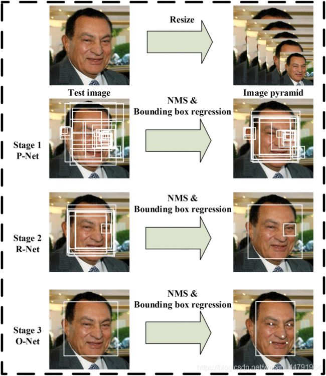
MTCNN,英文全称是Multi-task convolutional neural network,中文全称是多任务卷积神经网络,该神经网络将人脸区域检测与人脸关键点检测放在了一起。总体可分为P-Net、R-Net、和O-Net三层网络结构。
代码下载
https://github.com/bubbliiiing/mtcnn-keras
实现流程
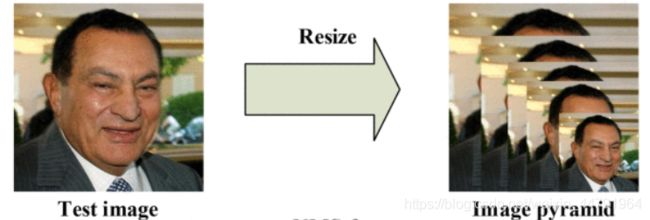
1、构建图像金字塔
首先将图像进行不同尺度的变换,构建图像金字塔,以适应不同大小的人脸的进行检测。
构建方式是通过不同的缩放系数factor对图片进行缩放,每次缩小为原来的factor大小。
实现示意图如下:
实现代码如下,当一个图片输入的时候,会缩放为不同大小的图片,但是缩小后的长宽最小不可以小于12:
#-----------------------------# # 计算原始输入图像 # 每一次缩放的比例 #-----------------------------# def calculateScales(img): copy_img = img.copy() pr_scale = 1.0 h,w,_ = copy_img.shape if min(w,h)>500: pr_scale = 500.0/min(h,w) w = int(w*pr_scale) h = int(h*pr_scale) elif max(w,h)<500: pr_scale = 500.0/max(h,w) w = int(w*pr_scale) h = int(h*pr_scale)scales = [] factor = 0.709 factor_count = 0 minl = min(h,w) while minl >= 12: scales.append(pr_scale*pow(factor, factor_count)) minl *= factor factor_count += 1 return scales
- 1
- 2
- 3
- 4
- 5
- 6
- 7
- 8
- 9
- 10
- 11
- 12
- 13
- 14
- 15
- 16
- 17
- 18
- 19
- 20
- 21
- 22
- 23
- 24
- 25
- 26
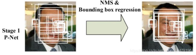
2、Pnet
Pnet的全称为Proposal Network,其基本的构造是一个全卷积网络。对上一步构建完成的图像金字塔,通过一个FCN进行初步特征提取与标定边框。
实现图片示意图如下:
Pnet的网络比较简单,实现代码如下:
#-----------------------------# # 粗略获取人脸框 # 输出bbox位置和是否有人脸 #-----------------------------# def create_Pnet(weight_path): input = Input(shape=[None, None, 3])x = Conv2D(10, (3, 3), strides=1, padding='valid', name='conv1')(input) x = PReLU(shared_axes=[1,2],name='PReLU1')(x) x = MaxPool2D(pool_size=2)(x) x = Conv2D(16, (3, 3), strides=1, padding='valid', name='conv2')(x) x = PReLU(shared_axes=[1,2],name='PReLU2')(x) x = Conv2D(32, (3, 3), strides=1, padding='valid', name='conv3')(x) x = PReLU(shared_axes=[1,2],name='PReLU3')(x) classifier = Conv2D(2, (1, 1), activation='softmax', name='conv4-1')(x) # 无激活函数,线性。 bbox_regress = Conv2D(4, (1, 1), name='conv4-2')(x) model = Model([input], [classifier, bbox_regress]) model.load_weights(weight_path, by_name=True) return model
- 1
- 2
- 3
- 4
- 5
- 6
- 7
- 8
- 9
- 10
- 11
- 12
- 13
- 14
- 15
- 16
- 17
- 18
- 19
- 20
- 21
- 22
- 23
- 24
在完成初步提取后,还需要进行Bounding-Box Regression调整窗口与NMS进行大部分窗口的过滤。
Pnet有两个输出,classifier用于判断这个网格点上的框的可信度,bbox_regress表示框的位置。
bbox_regress并不代表这个框在图片上的真实位置,如果需要将bbox_regress映射到真实图像上,还需要进行一次解码过程。
解码过程利用detect_face_12net函数实现,其实现步骤如下(需要配合代码理解):
1、判断哪些网格点的置信度较高,即该网格点内存在人脸。
2、记录该网格点的x,y轴。
3、利用函数计算bb1和bb2,分别代表图中框的左上角基点和右下角基点,二者之间差了11个像素,堆叠得到boundingbox 。
4、利用bbox_regress计算解码结果,解码公式为boundingbox = boundingbox + offset*12.0*scale。
简单理解就是Pnet的输出就是将整个网格分割成若干个网格点,;然后每个网格点初始状态下是一个11x11的框,这个由第三步得到;之后bbox_regress代表 每个网格点确定的框 的 左上角基点和右下角基点 的偏移情况。
#-------------------------------------# # 对pnet处理后的结果进行处理 #-------------------------------------# def detect_face_12net(cls_prob,roi,out_side,scale,width,height,threshold): cls_prob = np.swapaxes(cls_prob, 0, 1) roi = np.swapaxes(roi, 0, 2)stride = 0 # stride略等于2 if out_side != 1: stride = float(2*out_side-1)/(out_side-1) (x,y) = np.where(cls_prob>=threshold) boundingbox = np.array([x,y]).T # 找到对应原图的位置 bb1 = np.fix((stride * (boundingbox) + 0 ) * scale) bb2 = np.fix((stride * (boundingbox) + 11) * scale) # plt.scatter(bb1[:,0],bb1[:,1],linewidths=1) # plt.scatter(bb2[:,0],bb2[:,1],linewidths=1,c='r') # plt.show() boundingbox = np.concatenate((bb1,bb2),axis = 1) dx1 = roi[0][x,y] dx2 = roi[1][x,y] dx3 = roi[2][x,y] dx4 = roi[3][x,y] score = np.array([cls_prob[x,y]]).T offset = np.array([dx1,dx2,dx3,dx4]).T boundingbox = boundingbox + offset*12.0*scale rectangles = np.concatenate((boundingbox,score),axis=1) rectangles = rect2square(rectangles) pick = [] for i in range(len(rectangles)): x1 = int(max(0 ,rectangles[i][0])) y1 = int(max(0 ,rectangles[i][1])) x2 = int(min(width ,rectangles[i][2])) y2 = int(min(height,rectangles[i][3])) sc = rectangles[i][4] if x2>x1 and y2>y1: pick.append([x1,y1,x2,y2,sc]) return NMS(pick,0.3)
#-----------------------------#
# 将长方形调整为正方形
#-----------------------------#
def rect2square(rectangles):
w = rectangles[:,2] - rectangles[:,0]
h = rectangles[:,3] - rectangles[:,1]
l = np.maximum(w,h).T
rectangles[:,0] = rectangles[:,0] + w0.5 - l0.5
rectangles[:,1] = rectangles[:,1] + h0.5 - l0.5
rectangles[:,2:4] = rectangles[:,0:2] + np.repeat([l], 2, axis = 0).T
return rectangles
- 1
- 2
- 3
- 4
- 5
- 6
- 7
- 8
- 9
- 10
- 11
- 12
- 13
- 14
- 15
- 16
- 17
- 18
- 19
- 20
- 21
- 22
- 23
- 24
- 25
- 26
- 27
- 28
- 29
- 30
- 31
- 32
- 33
- 34
- 35
- 36
- 37
- 38
- 39
- 40
- 41
- 42
- 43
- 44
- 45
- 46
- 47
- 48
- 49
- 50
- 51
- 52
- 53
- 54
3、Rnet
Rnet全称为Refine Network,其基本的构造是一个卷积神经网络,相对于第一层的P-Net来说,增加了一个全连接层,因此对于输入数据的筛选会更加严格。在图片经过P-Net后,会留下许多预测窗口,我们将所有的预测窗口送入R-Net,这个网络会滤除大量效果比较差的候选框。
实现图片示意图如下:

实现代码如下:
#-----------------------------# # mtcnn的第二段 # 精修框 #-----------------------------# def create_Rnet(weight_path): input = Input(shape=[24, 24, 3]) # 24,24,3 -> 11,11,28 x = Conv2D(28, (3, 3), strides=1, padding='valid', name='conv1')(input) x = PReLU(shared_axes=[1, 2], name='prelu1')(x) x = MaxPool2D(pool_size=3,strides=2, padding='same')(x)# 11,11,28 -> 4,4,48 x = Conv2D(48, (3, 3), strides=1, padding='valid', name='conv2')(x) x = PReLU(shared_axes=[1, 2], name='prelu2')(x) x = MaxPool2D(pool_size=3, strides=2)(x) # 4,4,48 -> 3,3,64 x = Conv2D(64, (2, 2), strides=1, padding='valid', name='conv3')(x) x = PReLU(shared_axes=[1, 2], name='prelu3')(x) # 3,3,64 -> 64,3,3 x = Permute((3, 2, 1))(x) x = Flatten()(x) # 576 -> 128 x = Dense(128, name='conv4')(x) x = PReLU( name='prelu4')(x) # 128 -> 2 128 -> 4 classifier = Dense(2, activation='softmax', name='conv5-1')(x) bbox_regress = Dense(4, name='conv5-2')(x) model = Model([input], [classifier, bbox_regress]) model.load_weights(weight_path, by_name=True) return model
- 1
- 2
- 3
- 4
- 5
- 6
- 7
- 8
- 9
- 10
- 11
- 12
- 13
- 14
- 15
- 16
- 17
- 18
- 19
- 20
- 21
- 22
- 23
- 24
- 25
- 26
- 27
- 28
- 29
- 30
- 31
最后对选定的候选框进行Bounding-Box Regression和NMS进一步优化预测结果。
Rnet有两个输出,classifier用于判断这个网格点上的框的可信度,bbox_regress表示框的位置。
bbox_regress并不代表这个框在图片上的真实位置,如果需要将bbox_regress映射到真实图像上,还需要进行一次解码过程。
解码过程需要与Pnet的结果进行结合。在代码中,x1、y1、x2、y2代表由Pnet得到的图片在原图上的位置,w=x2-x1和h=y2-y1代表宽和高,bbox_regress与Pnet的结果结合的方式如下:
x1  = np.array([(x1+dx1*w)[0]]).T
y1  = np.array([(y1+dx2*h)[0]]).T
x2  = np.array([(x2+dx3*w)[0]]).T
y2  = np.array([(y2+dx4*h)[0]]).T
- 1
- 2
- 3
- 4
其中dx1、dx2、dy1、dy2就是Rnet获得的bbox_regress,实际上Rnet获得bbox_regress是长宽的缩小比例。
回归方法与Pnet不同,但是原理更加简单一些。
实现代码如下:
#-------------------------------------# # 对pnet处理后的结果进行处理 #-------------------------------------# def filter_face_24net(cls_prob,roi,rectangles,width,height,threshold):prob = cls_prob[:,1] pick = np.where(prob>=threshold) rectangles = np.array(rectangles) x1 = rectangles[pick,0] y1 = rectangles[pick,1] x2 = rectangles[pick,2] y2 = rectangles[pick,3] sc = np.array([prob[pick]]).T dx1 = roi[pick,0] dx2 = roi[pick,1] dx3 = roi[pick,2] dx4 = roi[pick,3] w = x2-x1 h = y2-y1 x1 = np.array([(x1+dx1*w)[0]]).T y1 = np.array([(y1+dx2*h)[0]]).T x2 = np.array([(x2+dx3*w)[0]]).T y2 = np.array([(y2+dx4*h)[0]]).T rectangles = np.concatenate((x1,y1,x2,y2,sc),axis=1) rectangles = rect2square(rectangles) pick = [] for i in range(len(rectangles)): x1 = int(max(0 ,rectangles[i][0])) y1 = int(max(0 ,rectangles[i][1])) x2 = int(min(width ,rectangles[i][2])) y2 = int(min(height,rectangles[i][3])) sc = rectangles[i][4] if x2>x1 and y2>y1: pick.append([x1,y1,x2,y2,sc]) return NMS(pick,0.3)
- 1
- 2
- 3
- 4
- 5
- 6
- 7
- 8
- 9
- 10
- 11
- 12
- 13
- 14
- 15
- 16
- 17
- 18
- 19
- 20
- 21
- 22
- 23
- 24
- 25
- 26
- 27
- 28
- 29
- 30
- 31
- 32
- 33
- 34
- 35
- 36
- 37
- 38
- 39
- 40
- 41
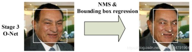
4、Onet
Onet与Rnet工作流程类似。
全称为Output Network,基本结构是一个较为复杂的卷积神经网络,相对于R-Net来说多了一个卷积层。O-Net的效果与R-Net的区别在于这一层结构会通过更多的监督来识别面部的区域,而且会对人的面部特征点进行回归,最终输出五个人脸面部特征点。
实现图片示意图如下:
实现代码如下:
#-----------------------------# # mtcnn的第三段 # 精修框并获得五个点 #-----------------------------# def create_Onet(weight_path): input = Input(shape = [48,48,3]) # 48,48,3 -> 23,23,32 x = Conv2D(32, (3, 3), strides=1, padding='valid', name='conv1')(input) x = PReLU(shared_axes=[1,2],name='prelu1')(x) x = MaxPool2D(pool_size=3, strides=2, padding='same')(x) # 23,23,32 -> 10,10,64 x = Conv2D(64, (3, 3), strides=1, padding='valid', name='conv2')(x) x = PReLU(shared_axes=[1,2],name='prelu2')(x) x = MaxPool2D(pool_size=3, strides=2)(x) # 8,8,64 -> 4,4,64 x = Conv2D(64, (3, 3), strides=1, padding='valid', name='conv3')(x) x = PReLU(shared_axes=[1,2],name='prelu3')(x) x = MaxPool2D(pool_size=2)(x) # 4,4,64 -> 3,3,128 x = Conv2D(128, (2, 2), strides=1, padding='valid', name='conv4')(x) x = PReLU(shared_axes=[1,2],name='prelu4')(x) # 3,3,128 -> 128,12,12 x = Permute((3,2,1))(x)# 1152 -> 256 x = Flatten()(x) x = Dense(256, name='conv5') (x) x = PReLU(name='prelu5')(x) # 鉴别 # 256 -> 2 256 -> 4 256 -> 10 classifier = Dense(2, activation='softmax',name='conv6-1')(x) bbox_regress = Dense(4,name='conv6-2')(x) landmark_regress = Dense(10,name='conv6-3')(x) model = Model([input], [classifier, bbox_regress, landmark_regress]) model.load_weights(weight_path, by_name=True) return model
- 1
- 2
- 3
- 4
- 5
- 6
- 7
- 8
- 9
- 10
- 11
- 12
- 13
- 14
- 15
- 16
- 17
- 18
- 19
- 20
- 21
- 22
- 23
- 24
- 25
- 26
- 27
- 28
- 29
- 30
- 31
- 32
- 33
- 34
- 35
- 36
- 37
- 38
- 39
最后对选定的候选框进行Bounding-Box Regression和NMS进一步优化预测结果。
Onet有三个输出,classifier用于判断这个网格点上的框的可信度,bbox_regress表示框的位置,landmark_regress表示脸上的五个标志点
bbox_regress并不代表这个框在图片上的真实位置,如果需要将bbox_regress映射到真实图像上,还需要进行一次解码过程。
解码过程需要与Rnet的结果进行结合。在代码中,x1、y1、x2、y2代表由Rnet得到的图片在原图上的位置,w=x2-x1和h=y2-y1代表宽和高,bbox_regress与Rnet的结果结合的方式如下:
x1  = np.array([(x1+dx1*w)[0]]).T
y1  = np.array([(y1+dx2*h)[0]]).T
x2  = np.array([(x2+dx3*w)[0]]).T
y2  = np.array([(y2+dx4*h)[0]]).T
- 1
- 2
- 3
- 4
其中dx1、dx2、dy1、dy2就是Onet获得的bbox_regress,实际上Onet获得bbox_regress是长宽的缩小比例。
实现代码如下:
#-------------------------------------# # 对onet处理后的结果进行处理 #-------------------------------------# def filter_face_48net(cls_prob,roi,pts,rectangles,width,height,threshold):prob = cls_prob[:,1] pick = np.where(prob>=threshold) rectangles = np.array(rectangles) x1 = rectangles[pick,0] y1 = rectangles[pick,1] x2 = rectangles[pick,2] y2 = rectangles[pick,3] sc = np.array([prob[pick]]).T dx1 = roi[pick,0] dx2 = roi[pick,1] dx3 = roi[pick,2] dx4 = roi[pick,3] w = x2-x1 h = y2-y1 pts0= np.array([(w*pts[pick,0]+x1)[0]]).T pts1= np.array([(h*pts[pick,5]+y1)[0]]).T pts2= np.array([(w*pts[pick,1]+x1)[0]]).T pts3= np.array([(h*pts[pick,6]+y1)[0]]).T pts4= np.array([(w*pts[pick,2]+x1)[0]]).T pts5= np.array([(h*pts[pick,7]+y1)[0]]).T pts6= np.array([(w*pts[pick,3]+x1)[0]]).T pts7= np.array([(h*pts[pick,8]+y1)[0]]).T pts8= np.array([(w*pts[pick,4]+x1)[0]]).T pts9= np.array([(h*pts[pick,9]+y1)[0]]).T x1 = np.array([(x1+dx1*w)[0]]).T y1 = np.array([(y1+dx2*h)[0]]).T x2 = np.array([(x2+dx3*w)[0]]).T y2 = np.array([(y2+dx4*h)[0]]).T rectangles=np.concatenate((x1,y1,x2,y2,sc,pts0,pts1,pts2,pts3,pts4,pts5,pts6,pts7,pts8,pts9),axis=1) pick = [] for i in range(len(rectangles)): x1 = int(max(0 ,rectangles[i][0])) y1 = int(max(0 ,rectangles[i][1])) x2 = int(min(width ,rectangles[i][2])) y2 = int(min(height,rectangles[i][3])) if x2>x1 and y2>y1: pick.append([x1,y1,x2,y2,rectangles[i][4], rectangles[i][5],rectangles[i][6],rectangles[i][7],rectangles[i][8],rectangles[i][9],rectangles[i][10],rectangles[i][11],rectangles[i][12],rectangles[i][13],rectangles[i][14]]) return NMS(pick,0.3)
- 1
- 2
- 3
- 4
- 5
- 6
- 7
- 8
- 9
- 10
- 11
- 12
- 13
- 14
- 15
- 16
- 17
- 18
- 19
- 20
- 21
- 22
- 23
- 24
- 25
- 26
- 27
- 28
- 29
- 30
- 31
- 32
- 33
- 34
- 35
- 36
- 37
- 38
- 39
- 40
- 41
- 42
- 43
- 44
- 45
- 46
- 47
- 48
- 49
- 50
- 51
- 52
最后得到的NMS(pick,0.3)就是识别出的人脸框的位置了。
mtcnn的效果
可以看出来效果还是非常好的。