吴恩达_Machine Learning_Programming Exercise 1: Linear Regression

1、Simple Octave / MATLAB function

（1）需要打开 “warmUpExercise.m”；

（2）输入：A = eye(5);

完整代码如下：

function A = warmUpExercise()
%WARMUPEXERCISE Example function in octave
%   A = WARMUPEXERCISE() is an example function that returns the 5x5 identity matrix

A = [];
% ============= YOUR CODE HERE ==============
% Instructions: Return the 5x5 identity matrix 
%               In octave, we return values by defining which variables
%               represent the return values (at the top of the file)
%               and then set them accordingly. 

A = eye(5);

% ===========================================


end

结果展示：

2、Linear regression with one variable

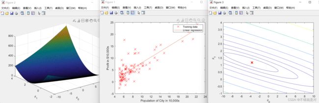
2.1 Plotting the Data

（1）打开 "plotData.m" ；

（2）输入：

plot(x, y, 'rx', 'MarkerSize', 10); % Plot the data
ylabel('Profit in $10,000s'); % Set the y−axis label
xlabel('Population of City in 10,000s'); % Set the x−axis label

完整代码如下：

function plotData(x, y)
%PLOTDATA Plots the data points x and y into a new figure 
%   PLOTDATA(x,y) plots the data points and gives the figure axes labels of
%   population and profit.

figure; % open a new figure window

% ====================== YOUR CODE HERE ======================
% Instructions: Plot the training data into a figure using the 
%               "figure" and "plot" commands. Set the axes labels using
%               the "xlabel" and "ylabel" commands. Assume the 
%               population and revenue data have been passed in
%               as the x and y arguments of this function.
%
% Hint: You can use the 'rx' option with plot to have the markers
%       appear as red crosses. Furthermore, you can make the
%       markers larger by using plot(..., 'rx', 'MarkerSize', 10);

plot(x,y,'rx','MarkerSize',10);
% plot(x,y,“x型”红色的点,大小为10)
ylabel('Profit in $10,000s');
xlabel('Population of City in 10,000s');

% ============================================================

end

结果展示：

2.2 Gradient Descent

（1）Computing the cost J(θ)

---

Linear Regression Model:

当X 和 θ都为列向量时；

补充：

---

（1）打开 "computeCost.m" ；

（2）输入：

h = X * theta;
J = (h-y)'*(h-y)/(2*m); 

% 注意，这里是 X * theta 的原因是，补一列1之后，对应相乘得到的结果即为预测值h；

完整代码如下：

function J = computeCost(X, y, theta)
%COMPUTECOST Compute cost for linear regression
%   J = COMPUTECOST(X, y, theta) computes the cost of using theta as the
%   parameter for linear regression to fit the data points in X and y

% Initialize some useful values
m = length(y); % number of training examples

% You need to return the following variables correctly 

% ====================== YOUR CODE HERE ======================
% Instructions: Compute the cost of a particular choice of theta
%               You should set J to the cost.

h = X * theta;
J = (h-y)'*(h-y)/(2*m); 

% =========================================================================

end

结果展示：

（2）Gradient descent

---

Gradient descent algorithm

1、注意要同时更新；

2、α是学习率；

3、是J（θ）求偏导的结果； 

4、 = ；

5、

---

（1）打开 "gradientDescent.m" ；

（2）输入：

    x=(alpha*(1/m))*(X'*((X*theta)-y));
    theta=theta-x;

完整代码如下：

function [theta, J_history] = gradientDescent(X, y, theta, alpha, num_iters)
%GRADIENTDESCENT Performs gradient descent to learn theta
%   theta = GRADIENTDESCENT(X, y, theta, alpha, num_iters) updates theta by 
%   taking num_iters gradient steps with learning rate alpha

% Initialize some useful values
m = length(y); % number of training examples
J_history = zeros(num_iters, 1);

for iter = 1:num_iters

    % ====================== YOUR CODE HERE ======================
    % Instructions: Perform a single gradient step on the parameter vector
    %               theta. 
    %
    % Hint: While debugging, it can be useful to print out the values
    %       of the cost function (computeCost) and gradient here.
    %

    x=(alpha*(1/m))*(X'*((X*theta)-y));
    theta=theta-x;


    % ============================================================

    % Save the cost J in every iteration    
    J_history(iter) = computeCost(X, y, theta);

end

end

结果展示：

3、Linear regression with multiple variables

3.1 Feature Normalization

---

归一化公式：

是平均值；是标准差；

---

（1）打开 "featureNormalize.m" ；

（2）输入：

mu = mean(X);%存储X的平均数，这里应为1*2的矩阵
sigma = std(X);%存储X的方差，这里应为1*2的矩阵
X_norm(:,1) = (X(:,1)-mean(X(:,1)))/std(X(:,1));
X_norm(:,2) = (X(:,2)-mean(X(:,2)))/std(X(:,2));

完整代码如下：

function [X_norm, mu, sigma] = featureNormalize(X)
%FEATURENORMALIZE Normalizes the features in X 
%   FEATURENORMALIZE(X) returns a normalized version of X where
%   the mean value of each feature is 0 and the standard deviation
%   is 1. This is often a good preprocessing step to do when
%   working with learning algorithms.

% You need to set these values correctly

% ====================== YOUR CODE HERE ======================
% Instructions: First, for each feature dimension, compute the mean
%               of the feature and subtract it from the dataset,
%               storing the mean value in mu. Next, compute the 
%               standard deviation of each feature and divide
%               each feature by it's standard deviation, storing
%               the standard deviation in sigma. 
%
%               Note that X is a matrix where each column is a 
%               feature and each row is an example. You need 
%               to perform the normalization separately for 
%               each feature. 
%
% Hint: You might find the 'mean' and 'std' functions useful.
%       

mu = mean(X);%存储X的平均数，这里应为1*2的矩阵
sigma = std(X);%存储X的方差，这里应为1*2的矩阵
X_norm(:,1) = (X(:,1)-mean(X(:,1)))/std(X(:,1));
X_norm(:,2) = (X(:,2)-mean(X(:,2)))/std(X(:,2));

% ============================================================

end

3.2 ComputeCostMulti

和之前的一样：

（1）打开 "computeCostMulti.m" ;

（2）输入：

function J = computeCostMulti(X, y, theta)
%COMPUTECOSTMULTI Compute cost for linear regression with multiple variables
%   J = COMPUTECOSTMULTI(X, y, theta) computes the cost of using theta as the
%   parameter for linear regression to fit the data points in X and y

% Initialize some useful values
m = length(y); % number of training examples

% You need to return the following variables correctly 
J = 0;

% ====================== YOUR CODE HERE ======================
% Instructions: Compute the cost of a particular choice of theta
%               You should set J to the cost.


h =  X*theta;
J = (h-y)'*(h-y)/(2*m);


% =========================================================================

end

3.3 gradientDescentMulti

和之前一样：

（1）打开 "gradientDescentMulti.m" ；

（2）输入：

function [theta, J_history] = gradientDescentMulti(X, y, theta, alpha, num_iters)
%GRADIENTDESCENTMULTI Performs gradient descent to learn theta
%   theta = GRADIENTDESCENTMULTI(x, y, theta, alpha, num_iters) updates theta by
%   taking num_iters gradient steps with learning rate alpha

% Initialize some useful values
m = length(y); % number of training examples
J_history = zeros(num_iters, 1);

for iter = 1:num_iters

    % ====================== YOUR CODE HERE ======================
    % Instructions: Perform a single gradient step on the parameter vector
    %               theta. 
    %
    % Hint: While debugging, it can be useful to print out the values
    %       of the cost function (computeCostMulti) and gradient here.
    %

    x=(alpha*(1/m))*(X'*((X*theta)-y));
    theta=theta-x;

    % ============================================================

    % Save the cost J in every iteration    
    J_history(iter) = computeCostMulti(X, y, theta);

end

end

ex1_multi

%% Machine Learning Online Class
%  Exercise 1: Linear regression with multiple variables
%
%  Instructions
%  ------------
% 
%  This file contains code that helps you get started on the
%  linear regression exercise. 
%
%  You will need to complete the following functions in this 
%  exericse:
%
%     warmUpExercise.m
%     plotData.m
%     gradientDescent.m
%     computeCost.m
%     gradientDescentMulti.m
%     computeCostMulti.m
%     featureNormalize.m
%     normalEqn.m
%
%  For this part of the exercise, you will need to change some
%  parts of the code below for various experiments (e.g., changing
%  learning rates).
%

%% Initialization

%% ================ Part 1: Feature Normalization ================

%% Clear and Close Figures
clear ; close all; clc

fprintf('Loading data ...\n');

%% Load Data
data = load('ex1data2.txt');
X = data(:, 1:2);
y = data(:, 3);
m = length(y);

% Print out some data points
fprintf('First 10 examples from the dataset: \n');
fprintf(' x = [%.0f %.0f], y = %.0f \n', [X(1:10,:) y(1:10,:)]');

fprintf('Program paused. Press enter to continue.\n');
pause;

% Scale features and set them to zero mean
fprintf('Normalizing Features ...\n');

[X mu sigma] = featureNormalize(X);

% Add intercept term to X
X = [ones(m, 1) X];


%% ================ Part 2: Gradient Descent ================

% ====================== YOUR CODE HERE ======================
% Instructions: We have provided you with the following starter
%               code that runs gradient descent with a particular
%               learning rate (alpha). 
%
%               Your task is to first make sure that your functions - 
%               computeCost and gradientDescent already work with 
%               this starter code and support multiple variables.
%
%               After that, try running gradient descent with 
%               different values of alpha and see which one gives
%               you the best result.
%
%               Finally, you should complete the code at the end
%               to predict the price of a 1650 sq-ft, 3 br house.
%
% Hint: By using the 'hold on' command, you can plot multiple
%       graphs on the same figure.
%
% Hint: At prediction, make sure you do the same feature normalization.
%

fprintf('Running gradient descent ...\n');

% Choose some alpha value
alpha = 0.01;
num_iters = 400;

% Init Theta and Run Gradient Descent 
theta = zeros(3, 1);
[theta, J_history] = gradientDescentMulti(X, y, theta, alpha, num_iters);

% Plot the convergence graph
figure;
plot(1:numel(J_history), J_history, '-b', 'LineWidth', 2);
xlabel('Number of iterations');
ylabel('Cost J');

% Display gradient descent's result
fprintf('Theta computed from gradient descent: \n');
fprintf(' %f \n', theta);
fprintf('\n');

% Estimate the price of a 1650 sq-ft, 3 br house
% ====================== YOUR CODE HERE ======================
% Recall that the first column of X is all-ones. Thus, it does
% not need to be normalized.
price = [1,1650,3]*theta; % You should change this


% ============================================================

fprintf(['Predicted price of a 1650 sq-ft, 3 br house ' ...
         '(using gradient descent):\n $%f\n'], price);

fprintf('Program paused. Press enter to continue.\n');
pause;

%% ================ Part 3: Normal Equations ================

fprintf('Solving with normal equations...\n');

% ====================== YOUR CODE HERE ======================
% Instructions: The following code computes the closed form 
%               solution for linear regression using the normal
%               equations. You should complete the code in 
%               normalEqn.m
%
%               After doing so, you should complete this code 
%               to predict the price of a 1650 sq-ft, 3 br house.
%

%% Load Data
data = csvread('ex1data2.txt');
X = data(:, 1:2);
y = data(:, 3);
m = length(y);

% Add intercept term to X
X = [ones(m, 1) X];

% Calculate the parameters from the normal equation
theta = normalEqn(X, y);

% Display normal equation's result
fprintf('Theta computed from the normal equations: \n');
fprintf(' %f \n', theta);
fprintf('\n');


% Estimate the price of a 1650 sq-ft, 3 br house
% ====================== YOUR CODE HERE ======================
price = [1,1650,3]*theta; % You should change this


% ============================================================

fprintf(['Predicted price of a 1650 sq-ft, 3 br house ' ...
         '(using normal equations):\n $%f\n'], price);

4、NormalEqn

---

 

---

function [theta] = normalEqn(X, y)
%NORMALEQN Computes the closed-form solution to linear regression 
%   NORMALEQN(X,y) computes the closed-form solution to linear 
%   regression using the normal equations.

theta = zeros(size(X, 2), 1);

% ====================== YOUR CODE HERE ======================
% Instructions: Complete the code to compute the closed form solution
%               to linear regression and put the result in theta.
%

% ---------------------- Sample Solution ----------------------

theta = inv(X'*X)*X'*y;


% -------------------------------------------------------------


% ============================================================

end