【Numpy】北理工python数据分析之Numpy学习笔记
Numpy
因为要学pytorch,准备重学下numpy,第一次是本科的时候看的,印象不深刻,顺便做做笔记以便以后复习。
学习资料来自MOOC北理工嵩天老师的Python数据分析与展示,链接放在下面。
在Ubuntu20.04中使用anaconda3进行学习。其中numpy版本为1.22.3。学习工具有ipython。
Have fun!
课程链接:Python数据分析与展示
Ipython魔术指令
在Ipython中有一些魔术指令,熟悉以下给学习带来便捷
首先,Ipython可以使用shell的一些基本命令,不做举例。
魔术指令:
#输入magic,弹出魔术指令help文档
%magic#同上
%hist#显示历史输入
%pdb#当陷入异常时自动进入pdb调试器
%reset#删除当前所有变量
%who#显示ipython中的所有定义的变量
%time statement#给出代码执行时间,statement表示一段代码
%timeit statement#多次执行代码,计算综合平均时间
引入Numpy
引入Numpy包的默认方法
import numpy as np
Numpy入门
ndarray和普通数据结构列表的区别
#!/usr/bin/python3

def pySum():
	a = [0, 1, 2, 3, 4]
	b = [9, 8, 7, 6, 5]
	c = []

	for i in range(len(a)):
		c.append(a[i]**2 + b[i]**3)

	return c

import numpy as np

def npSum():
	a = np.array([0, 1, 2, 3, 4])
	b = np.array([9, 8, 7, 6, 5])

	c = a**2 + b**3

	return c

print(pySum())
print(npSum())
pySum函数计算列表a,b返回结果。而npSum函数则是pySum函数的numpy版本。可以看到numpy版本简单许多,并且不需要用到循环,numpy底层是用c语言实现的,效率很高。
运行结果:
[729, 513, 347, 225, 141]
[729 513 347 225 141]
ndarray的属性
以下矩阵其实是数组,因为上面的程序进行的是数组运算
| attributes | meanings |
|---|---|
| .ndim | 矩阵的秩 |
| .shape | 矩阵的形状,以元组呈现 |
| .size | 矩阵的所含元素个数 |
| .dtype | 矩阵中数据类型 |
| .itemsize | 矩阵中每个数据所占内存大小 |
ipython中验证:
n [1]: import numpy as np

In [2]: a = np.array([[0, 1, 2, 3, 4], [9, 8, 7, 6, 5]])

In [3]: a.ndim
Out[3]: 2

In [4]: a.shape
Out[4]: (2, 5)

In [5]: a.size
Out[5]: 10

In [6]: a.dtype
Out[6]: dtype('int64')

In [7]: a.itemsize
Out[7]: 8
array中的数据也可以不同质,但是会有想不到的麻烦,在处理大量数据时不建议使用。
In [8]: x = np.array([[0, 1, 2, 3, 4], [9, 8, 7, 6]])

In [9]: x.ndim
Out[9]: 1

In [10]: x.shape
Out[10]: (2,) #shape是很奇怪的元组

In [11]: x.size
Out[11]: 2	#size也只是2,与同质的矩阵不同

In [12]: x.dtype
Out[12]: dtype('O') #这里数据类型是‘O’,就是对象

In [13]: x.itemsize
Out[13]: 8
ndarray的创建
-
从列表,元组,列表元组混合创建
x = np.array(list/tuple)
x = np.array(list/tuple, dtype=np.float64)
当不指定dtype时,数据类型是numpy中默认的类型,一般是float64
In [64]: x = np.array([0, 1, 2, 3])#从列表创建 In [65]: print(x) [0 1 2 3] In [66]: x = np.array((4, 5, 6, 7))#从元组创建 In [67]: print(x) [4 5 6 7] In [68]: x = np.array([[1, 2], [9, 8], (0.1, 0.2)])#从列表元组混合创建 In [69]: print(x) [[1. 2. ] [9. 8. ] [0.1 0.2]] -
从numpy提供的函数创建
1.首先是一些无中生有的方法
function comment np.arange(n) 类似range函数,生成从0到n的元素 np.ones(shape) shape是元组,根据shape生成一个全一数组 np.zeros(shape) shape是元组,根据shape生成一个全0数组 np.full(shape, val) 根据shape生成一个数组,每个元素都为val np.eye(n) 创建一个n维单位阵 In [71]: np.arange(10) Out[71]: array([0, 1, 2, 3, 4, 5, 6, 7, 8, 9]) In [72]: np.ones((3,6)) Out[72]: array([[1., 1., 1., 1., 1., 1.], [1., 1., 1., 1., 1., 1.], [1., 1., 1., 1., 1., 1.]]) In [73]: np.zeros((3,6), dtype=np.int32) Out[73]: array([[0, 0, 0, 0, 0, 0], [0, 0, 0, 0, 0, 0], [0, 0, 0, 0, 0, 0]], dtype=int32) In [74]: np.eye(5) Out[74]: array([[1., 0., 0., 0., 0.], [0., 1., 0., 0., 0.], [0., 0., 1., 0., 0.], [0., 0., 0., 1., 0.], [0., 0., 0., 0., 1.]]) In [75]: x = np.ones((2, 3, 4))#数组的数组思想 In [76]: print(x) [[[1. 1. 1. 1.] [1. 1. 1. 1.] [1. 1. 1. 1.]] [[1. 1. 1. 1.] [1. 1. 1. 1.] [1. 1. 1. 1.]]] In [77]: x.shape Out[77]: (2, 3, 4)2.再是一些根据已有的数据生成数组的方法
function comment np.ones_like(a) 根据a的形状生成一个全1数组 np.zeros_like(a) 根据a的形状生成一个全0数组 np.full_like(a, val) 根据a的形状生成一个数组,元素都为val 3.其他方法
function comment np.linspace() 根据起止数等间距填充数据,形成数组 np.concatenate() 将两个或多个数组合并成一个新数组 In [79]: a = np.linspace(1, 10 ,4) In [80]: a Out[80]: array([ 1., 4., 7., 10.]) In [81]: b = np.linspace(1, 10 , 4, endpoint=False) In [82]: b Out[82]: array([1. , 3.25, 5.5 , 7.75]) #endpoint表示最后一个数是否在生成的数组中的最后一个元素上In [84]: c = np.concatenate((a, b)) In [85]: c Out[85]: array([ 1. , 4. , 7. , 10. , 1. , 3.25, 5.5 , 7.75]) -
从字节流创建,从文件读取数据创建
ndarray维度变换
| function | comment |
|---|---|
| .reshape(shape) | 不改变数组元素,返回一个shape形状的数组,原数组不变 |
| .resize(shape) | 与reshape相似,但是改变原数组,返回引用 |
| .swapaxes(ax1, ax2) | 将数组n个维度中两个交换 |
| .flatten() | 对数组降维,降成一维 |
In [87]: a = np.ones((2, 3, 4), dtype=np.int32)

In [88]: a.reshape((3,8))
Out[88]:
array([[1, 1, 1, 1, 1, 1, 1, 1],
       [1, 1, 1, 1, 1, 1, 1, 1],
       [1, 1, 1, 1, 1, 1, 1, 1]], dtype=int32)

In [89]: a
Out[89]:
array([[[1, 1, 1, 1],
        [1, 1, 1, 1],
        [1, 1, 1, 1]],

       [[1, 1, 1, 1],
        [1, 1, 1, 1],
        [1, 1, 1, 1]]], dtype=int32)
注意:这里的a数组并没有发生变化
In [90]: a.resize((3,8))

In [91]: a
Out[91]:
array([[1, 1, 1, 1, 1, 1, 1, 1],
       [1, 1, 1, 1, 1, 1, 1, 1],
       [1, 1, 1, 1, 1, 1, 1, 1]], dtype=int32)
这里a已经改变了
In [92]: a.flatten()
Out[92]:
array([1, 1, 1, 1, 1, 1, 1, 1, 1, 1, 1, 1, 1, 1, 1, 1, 1, 1, 1, 1, 1, 1,
       1, 1], dtype=int32)
这里a直接降至一维
ndarray类型转换
-
数组内数据类型的转换
直接上代码:
In [97]: a = np.ones((2, 3, 4), dtype=np.int) In [98]: a Out[98]: array([[[1, 1, 1, 1], [1, 1, 1, 1], [1, 1, 1, 1]], [[1, 1, 1, 1], [1, 1, 1, 1], [1, 1, 1, 1]]]) In [99]: b = a.astype(np.float) In [100]: b Out[100]: array([[[1., 1., 1., 1.], [1., 1., 1., 1.], [1., 1., 1., 1.]], [[1., 1., 1., 1.], [1., 1., 1., 1.], [1., 1., 1., 1.]]])astype(new_type), 该方法一定会生成一个新的数组,拷贝了原数组然后进行了数据类型的改变。
-
ndarray数组向列表的转换
使用tolist方法
In [104]: a = np.full((2, 3, 4), 25, dtype=np.int32)

In [105]: a
Out[105]:
array([[[25, 25, 25, 25],
        [25, 25, 25, 25],
        [25, 25, 25, 25]],

       [[25, 25, 25, 25],
        [25, 25, 25, 25],
        [25, 25, 25, 25]]], dtype=int32)

In [106]: a.tolist()
Out[106]:
[[[25, 25, 25, 25], [25, 25, 25, 25], [25, 25, 25, 25]],
 [[25, 25, 25, 25], [25, 25, 25, 25], [25, 25, 25, 25]]]
返回的是一个列表,原数组不改变
ndarray索引与切片
-
一位数组索引切片与列表相同
In [11]: a = np.array([9, 8, 7, 6, 5]) In [12]: a[2] Out[12]: 7 In [13]: a[1 : 4 : 2] Out[13]: array([8, 6]) -
多维数组的操作也大同小异
#首先建立一个2*3*4的数组
In [14]: a = np.arange(24).reshape((2, 3, 4))

In [15]: a
Out[15]:
array([[[ 0,  1,  2,  3],
        [ 4,  5,  6,  7],
        [ 8,  9, 10, 11]],

       [[12, 13, 14, 15],
        [16, 17, 18, 19],
        [20, 21, 22, 23]]])
注意py里的索引都是在一个中括号内完成的,不是数组数组的概念
In [17]: a[1, 2, 3]
Out[17]: 23

In [18]: a[0, 1, 2]
Out[18]: 6

In [19]: a[-1, -2, -3]
Out[19]: 17
切片操作
In [21]: a[:, 1, -3]
Out[21]: array([ 5, 17])

In [22]: a[:, 1:3, :]
Out[22]:
array([[[ 4,  5,  6,  7],
        [ 8,  9, 10, 11]],

       [[16, 17, 18, 19],
        [20, 21, 22, 23]]])

In [23]: a[:, :, ::2]
Out[23]:
array([[[ 0,  2],
        [ 4,  6],
        [ 8, 10]],

       [[12, 14],
        [16, 18],
        [20, 22]]])
ndarray数组运算
-
数组与标量的运算
举个例子:求a的平均值
In [10]: a = np.arange(24).reshape((2, 3, 4))

In [11]: a.mean()
Out[11]: 11.5

In [12]: a/a.mean()
Out[12]:
array([[[0.        , 0.08695652, 0.17391304, 0.26086957],
        [0.34782609, 0.43478261, 0.52173913, 0.60869565],
        [0.69565217, 0.7826087 , 0.86956522, 0.95652174]],

       [[1.04347826, 1.13043478, 1.2173913 , 1.30434783],
        [1.39130435, 1.47826087, 1.56521739, 1.65217391],
        [1.73913043, 1.82608696, 1.91304348, 2.        ]]])
numpy一元函数(只有一个数组参与的函数)
function comment np.abs(x) np.fabs(x) 计算数组各元素的绝对值 np.sqrt(x) 计算数组各元素的平方根 np.square(x) 计算数组各元素的平方 np.log(x) np.log10(x) np.log2(x) 计算数组各元素的自然对数,10底对数,2底对数 np.ceil(x) np.floor(x) 计算数组各元素的向上取整和向下取整 np.ring(x) 计算数组各元素的四舍五入 np.modf(x) 将数组的整数部分和小数部分分别返回,但是结果都是浮点数组 np.三角函数 计算各元素的指数值 np.sign(x) 符号函数,取符号数组 老油条看到这么多数学函数,不要怕,用到的时候再看就好了
举几个例子:
In [13]: np.square(a)
Out[13]:
array([[[  0,   1,   4,   9],
        [ 16,  25,  36,  49],
        [ 64,  81, 100, 121]],

       [[144, 169, 196, 225],
        [256, 289, 324, 361],
        [400, 441, 484, 529]]])

In [14]: a = np.sqrt(a)

In [15]: a
Out[15]:
array([[[0.        , 1.        , 1.41421356, 1.73205081],
        [2.        , 2.23606798, 2.44948974, 2.64575131],
        [2.82842712, 3.        , 3.16227766, 3.31662479]],

       [[3.46410162, 3.60555128, 3.74165739, 3.87298335],
        [4.        , 4.12310563, 4.24264069, 4.35889894],
        [4.47213595, 4.58257569, 4.69041576, 4.79583152]]])

In [16]: np.modf(a)
Out[16]:
(array([[[0.        , 0.        , 0.41421356, 0.73205081],
         [0.        , 0.23606798, 0.44948974, 0.64575131],
         [0.82842712, 0.        , 0.16227766, 0.31662479]],

        [[0.46410162, 0.60555128, 0.74165739, 0.87298335],
         [0.        , 0.12310563, 0.24264069, 0.35889894],
         [0.47213595, 0.58257569, 0.69041576, 0.79583152]]]),
 array([[[0., 1., 1., 1.],
         [2., 2., 2., 2.],
         [2., 3., 3., 3.]],

        [[3., 3., 3., 3.],
         [4., 4., 4., 4.],
         [4., 4., 4., 4.]]]))#这里的结果注意一下,两个数组都是浮点数类型的
需要注意的是这些一元函数都不会返回引用,所以都需要赋值才行
-
二元函数
function comment + - * / ** np.maximum(x, y) np.fmax() np.minimum(x, y) np.fmin() 元素级的最值 np.mod(x, y) 元素级的模运算 np.copysign(x, y) 将数组y中的各元素符号赋值给数组x对应的元素 > < >= <= == != 算术比较,产生bool型数组 In [17]: a = np.arange(24).reshape((2, 3, 4)) In [18]: b = np.sqrt(a) In [19]: a Out[19]: array([[[ 0, 1, 2, 3], [ 4, 5, 6, 7], [ 8, 9, 10, 11]], [[12, 13, 14, 15], [16, 17, 18, 19], [20, 21, 22, 23]]]) In [20]: b Out[20]: array([[[0. , 1. , 1.41421356, 1.73205081], [2. , 2.23606798, 2.44948974, 2.64575131], [2.82842712, 3. , 3.16227766, 3.31662479]], [[3.46410162, 3.60555128, 3.74165739, 3.87298335], [4. , 4.12310563, 4.24264069, 4.35889894], [4.47213595, 4.58257569, 4.69041576, 4.79583152]]]) In [22]: np.maximum(a, b) Out[22]: array([[[ 0., 1., 2., 3.], [ 4., 5., 6., 7.], [ 8., 9., 10., 11.]], [[12., 13., 14., 15.], [16., 17., 18., 19.], [20., 21., 22., 23.]]]) In [23]: a > b Out[23]: array([[[False, False, True, True], [ True, True, True, True], [ True, True, True, True]], [[ True, True, True, True], [ True, True, True, True], [ True, True, True, True]]])
Numpy数据存取
CSV文件格式
CSV(Comma-Separated Value,逗号分隔值)
用来存储批量数据,以逗号分隔同一行的数据
numpy中读写文件函数
np.savetxt() np.loadtxt()
首先savetxt()函数:
np.savetxt(frame, array, fmt='%.18e', delimiter=None)
'''
frame: 文件,字符串或者生成器,可以是.gz或者.bz2的压缩文件。
array:存入文件的数组
fmt:存入的格式
delimiter:分隔符,None就是默认任何空格,在CSV中一定得是逗号
'''
举例:
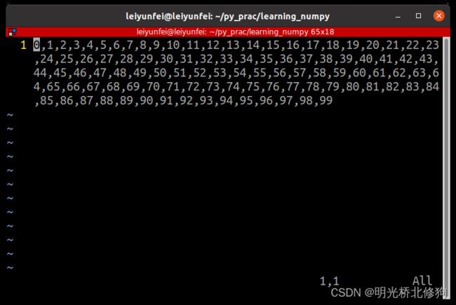
In [13]: a = np.arange(100).reshape((5, 20))
In [14]: np.savetxt('a.csv', a, fmt="%d", delimiter=",")
打开a.csv看看

再存一个浮点数的看看:
In [17]: np.savetxt('b.csv', a, fmt="%.1f", delimiter=",")

loadtxt()函数:
np.loadtxt(frame, dtype=np.float, delimiter=None, unpack=False)
'''
frame:文件,字符串或者产生器,可以是gz bz2压缩文件
dtype:数据类型,可选。默认是float类型
delimiter:分割字符串,默认是任何空格
unpack:如果为真,读入属性将分别写入不同的变量
'''
In [18]: np.loadtxt('a.csv', delimiter=',')
Out[18]:
array([[ 0.,  1.,  2.,  3.,  4.,  5.,  6.,  7.,  8.,  9., 10., 11., 12.,
        13., 14., 15., 16., 17., 18., 19.],
       [20., 21., 22., 23., 24., 25., 26., 27., 28., 29., 30., 31., 32.,
        33., 34., 35., 36., 37., 38., 39.],
       [40., 41., 42., 43., 44., 45., 46., 47., 48., 49., 50., 51., 52.,
        53., 54., 55., 56., 57., 58., 59.],
       [60., 61., 62., 63., 64., 65., 66., 67., 68., 69., 70., 71., 72.,
        73., 74., 75., 76., 77., 78., 79.],
       [80., 81., 82., 83., 84., 85., 86., 87., 88., 89., 90., 91., 92.,
        93., 94., 95., 96., 97., 98., 99.]])
In [21]: b = np.loadtxt('a.csv', dtype=np.int32, delimiter=',')

In [22]: b
Out[22]:
array([[ 0,  1,  2,  3,  4,  5,  6,  7,  8,  9, 10, 11, 12, 13, 14, 15,
        16, 17, 18, 19],
       [20, 21, 22, 23, 24, 25, 26, 27, 28, 29, 30, 31, 32, 33, 34, 35,
        36, 37, 38, 39],
       [40, 41, 42, 43, 44, 45, 46, 47, 48, 49, 50, 51, 52, 53, 54, 55,
        56, 57, 58, 59],
       [60, 61, 62, 63, 64, 65, 66, 67, 68, 69, 70, 71, 72, 73, 74, 75,
        76, 77, 78, 79],
       [80, 81, 82, 83, 84, 85, 86, 87, 88, 89, 90, 91, 92, 93, 94, 95,
        96, 97, 98, 99]], dtype=int32)
缺点是这两个函数只能操作一维二维的数组
多维数据的存取
tofile()函数
a.tofile(frmae, sep='', format='%s')
'''
frame:文件,字符串。
sep:数据分割字符串,如果是空串,写入文件为二进制
format:写入数据的格式
'''
In [26]: a = np.arange(100).reshape(5, 10, 2)

In [27]: a.tofile("b.data", sep=",", format="%d")
打开如下:
如果
In [28]: a.tofile('b.data', format="%d")
将是乱码
fromfile函数:
np.fromfile(frame, dtype=float, count=-1, sep='')
'''
frame:文件,字符串
dtype:读取的数据类型
count:读入元素个数,默认-1表示整个文件
sep:分隔符,同上,空串表示二进制
'''
In [29]: a = np.arange(100).reshape(5, 10, 2)

In [30]: a.tofile('b.data', sep=",", format="%d")

In [31]: c = np.fromfile("b.data", dtype=np.int32, sep=",")

In [32]: c
Out[32]:
array([ 0,  1,  2,  3,  4,  5,  6,  7,  8,  9, 10, 11, 12, 13, 14, 15, 16,
       17, 18, 19, 20, 21, 22, 23, 24, 25, 26, 27, 28, 29, 30, 31, 32, 33,
       34, 35, 36, 37, 38, 39, 40, 41, 42, 43, 44, 45, 46, 47, 48, 49, 50,
       51, 52, 53, 54, 55, 56, 57, 58, 59, 60, 61, 62, 63, 64, 65, 66, 67,
       68, 69, 70, 71, 72, 73, 74, 75, 76, 77, 78, 79, 80, 81, 82, 83, 84,
       85, 86, 87, 88, 89, 90, 91, 92, 93, 94, 95, 96, 97, 98, 99],
      dtype=int32)
注意:这里fromfile读取进入数组后,数组都是一维的,一般使用reshape进行维度变换
这里进行一个二进制格式存取的演示,并且使用reshape将读入的数组进行变维:
In [40]: a.tofile('b.data', format='%d')

In [41]: c = np.fromfile('b.data', dtype=np.int64).reshape(5, 10, 2)

In [42]: c
Out[42]:
array([[[ 0,  1],
        [ 2,  3],
        [ 4,  5],
        [ 6,  7],
        [ 8,  9],
        [10, 11],
        [12, 13],
        [14, 15],
        [16, 17],
        [18, 19]],

       [[20, 21],
        [22, 23],
        [24, 25],
        [26, 27],
        [28, 29],
        [30, 31],
        [32, 33],
        [34, 35],
        [36, 37],
        [38, 39]],

       [[40, 41],
        [42, 43],
        [44, 45],
        [46, 47],
        [48, 49],
        [50, 51],
        [52, 53],
        [54, 55],
        [56, 57],
        [58, 59]],

       [[60, 61],
        [62, 63],
        [64, 65],
        [66, 67],
        [68, 69],
        [70, 71],
        [72, 73],
        [74, 75],
        [76, 77],
        [78, 79]],

       [[80, 81],
        [82, 83],
        [84, 85],
        [86, 87],
        [88, 89],
        [90, 91],
        [92, 93],
        [94, 95],
        [96, 97],
        [98, 99]]])
注意:使用这一对方法,需要知道数组的维度,一般会再写一个文件存储数组相关信息。
Numpy特有的存取方法
save,savez与load
np.save(frame, array)
np.savez(frame, array)
np.load(frame)
'''
frame:文件名,以.npy为扩展名,压缩扩展名为.npz
array:数组变量
'''
In [44]: np.save("a.npy", a)

In [45]: b = np.load("a.npy")

In [46]: b
Out[46]:
array([[[ 0,  1],
        [ 2,  3],
        [ 4,  5],
        [ 6,  7],
        [ 8,  9],
        [10, 11],
        [12, 13],
        [14, 15],
        [16, 17],
        [18, 19]],

       [[20, 21],
        [22, 23],
        [24, 25],
        [26, 27],
        [28, 29],
        [30, 31],
        [32, 33],
        [34, 35],
        [36, 37],
        [38, 39]],

       [[40, 41],
        [42, 43],
        [44, 45],
        [46, 47],
        [48, 49],
        [50, 51],
        [52, 53],
        [54, 55],
        [56, 57],
        [58, 59]],

       [[60, 61],
        [62, 63],
        [64, 65],
        [66, 67],
        [68, 69],
        [70, 71],
        [72, 73],
        [74, 75],
        [76, 77],
        [78, 79]],

       [[80, 81],
        [82, 83],
        [84, 85],
        [86, 87],
        [88, 89],
        [90, 91],
        [92, 93],
        [94, 95],
        [96, 97],
        [98, 99]]])
为什么可以直接打开不提供维度信息?

因为npy文件第一行中指明了数组相关信息
Numpy 随机数相关功能
numpy子库random提供相关的功能
| function | comment |
|---|---|
| rand(d0, d1…dn) | 根据d0-dn创建随机数数组,浮点数,[0, 1),均匀分布 |
| randn(d0, d1…dn) | 根据d0-dn创建随机数数组,标准正态分布 |
| randint(low [, high, shape]) | 根据shape创建随机整数或整数数组,范围是[low,high) |
| seed(s) | 随机数种子,s是给定的种子值 |
In [1]: import numpy as np

In [2]: a = np.random.rand(3, 4, 5)#生成3*4*5的随机数数组,范围0~1,1取不到,均匀分布

In [3]: a
Out[3]:
array([[[0.22855554, 0.53895778, 0.8990956 , 0.03460846, 0.80936432],
        [0.38602525, 0.95082778, 0.25007749, 0.88049274, 0.94852455],
        [0.37985729, 0.05092291, 0.12991747, 0.79304105, 0.29923155],
        [0.63284688, 0.90729409, 0.68672494, 0.58729567, 0.65911695]],

       [[0.74592831, 0.0769337 , 0.40885755, 0.67209545, 0.88724064],
        [0.16406816, 0.12169161, 0.86875681, 0.02115887, 0.12646621],
        [0.22963925, 0.31762675, 0.59551248, 0.77621544, 0.02643761],
        [0.1202724 , 0.50328377, 0.16150334, 0.29160171, 0.93511997]],

       [[0.536302  , 0.72972245, 0.62452992, 0.81509939, 0.25614635],
        [0.85667339, 0.4896346 , 0.44260732, 0.02752194, 0.94911712],
        [0.57801131, 0.24271987, 0.97145063, 0.43145098, 0.38722077],
        [0.62954656, 0.5970487 , 0.92360391, 0.80155753, 0.71069473]]])

In [4]: sn = np.random.randn(3, 4, 5) #正态分布

In [5]: sn
Out[5]:
array([[[-0.80285747, -0.53518958,  0.38004255, -0.99689688,
          0.13284149],
        [ 0.64754759,  1.6824004 ,  1.96022306,  0.66429774,
          0.38430592],
        [ 1.15564303,  0.15239773,  0.74341428, -1.36023864,
          0.76729678],
        [ 1.74108334,  2.23838781, -0.56746454, -0.4348884 ,
          0.09969999]],

       [[ 0.65061914,  1.51382457, -1.03026261, -0.55293345,
          0.51808715],
        [-0.1243385 ,  0.35084291,  0.49323145, -0.97200827,
          0.13647158],
        [-1.59078417, -0.62574367, -0.23666443, -1.95238941,
          0.91223346],
        [ 0.80295509, -0.17089901,  0.48476418, -0.48047162,
         -0.24084512]],

       [[ 1.03365949,  0.13828344,  1.47268197,  0.17788982,
         -0.06274534],
        [-0.04690676,  0.01632059, -0.11124271, -0.40165229,
          1.42563916],
        [ 1.75412661,  2.3482051 , -0.29734503,  0.3106709 ,
          0.66124406],
        [-1.64166232, -0.17699444, -1.1448258 , -0.59836659,
         -0.16537533]]])

In [6]: b = np.random.randint(100, 200, (3, 4))# 生成100~200的整数随机数数组,3*4维

In [7]: b
Out[7]:
array([[120, 130, 192, 185],
       [114, 109, 126, 111],
       [125, 184, 121, 185]])

In [8]: np.random.seed(10)#指定随机数种子,种子相同,生成的伪随机数数组完全相同

In [9]: np.random.randint(100, 200, (3, 4))
Out[9]:
array([[109, 115, 164, 128],
       [189, 193, 129, 108],
       [173, 100, 140, 136]])

In [10]: np.random.randint(100, 200, (3, 4))
Out[10]:
array([[116, 111, 154, 188],
       [162, 133, 172, 178],
       [149, 151, 154, 177]])

In [11]: np.random.seed(10)

In [12]: np.random.randint(100, 200, (3, 4))
Out[12]:
array([[109, 115, 164, 128],
       [189, 193, 129, 108],
       [173, 100, 140, 136]])
还有
| function | comment |
|---|---|
| shuffle(a) | 根据数组a的第一轴进行随机排列,改变a |
| permutation(a) | 根据数组a的第一轴产生一个新的乱序数组,不改变a |
| choice(a [, size, replace, p]) | 从一维数组a中以概率p抽取元素,形成size形状数组replace表示是否可以重用元素,默认为False |
In [16]: a = np.random.randint(100, 200, (3, 4))#shuffle()

In [17]: a
Out[17]:
array([[111, 154, 188, 162],
       [133, 172, 178, 149],
       [151, 154, 177, 169]])

In [18]: np.random.shuffle(a)

In [19]: a
Out[19]:
array([[111, 154, 188, 162],
       [151, 154, 177, 169],
       [133, 172, 178, 149]])

In [19]: a
Out[19]:
array([[111, 154, 188, 162],
       [151, 154, 177, 169],
       [133, 172, 178, 149]])

In [20]: np.random.permutation(a)#permutation()
Out[20]:
array([[133, 172, 178, 149],
       [111, 154, 188, 162],
       [151, 154, 177, 169]])

In [21]: a
Out[21]:
array([[111, 154, 188, 162],
       [151, 154, 177, 169],
       [133, 172, 178, 149]])

In [22]: b = np.random.randint(100, 200, (8,))#choice()

In [23]: b
Out[23]: array([113, 192, 186, 130, 130, 189, 112, 165])

In [24]: np.random.choice(b, (3, 2))
Out[24]:
array([[165, 192],
       [130, 130],
       [186, 189]])

In [25]: np.random.choice(b, (3, 2), replace=False)#不可重复抽取
Out[25]:
array([[192, 130],
       [186, 165],
       [130, 113]])

In [26]: np.random.choice(b, (3, 2), p = b/np.sum(b))#这里元素值越大,被抽取的概率越高
Out[26]:
array([[130, 186],
       [130, 113],
       [112, 130]])
产生分布的函数:
| function | comment |
|---|---|
| uniform(low, high, size) | 产生具有均匀分布的数组,low—high指定起始终止,size指定形状 |
| normal(loc, scale, size) | 正态分布,loc均值,scale标准差,size形状 |
| poisson(lam, size) | 泊松分布,lam随机事件发生率,size形状 |
复习完概率论再看看吧
Numpy 统计函数介绍
函数是库级别的,也就是可以通过静态np直接调用
| function | comment |
|---|---|
| sum(a, axis=None) | 根据给定轴计算数组a相关元素之和,axis是整数或者元组 |
| mean(a, axis=None) | 根据给定轴计算数组a相关元素的期望,axis同上 |
| average(a, axis=None, weights=None) | 根据给定轴计算数组a相关元素的加权平均值 |
| std(a, axis=None) | 标准差 |
| var(a, axis=None) | 方差 |
上例子:
In [1]: import numpy as np

In [2]: a = np.arange(15).reshape(3, 5)

In [3]: a
Out[3]:
array([[ 0,  1,  2,  3,  4],
       [ 5,  6,  7,  8,  9],
       [10, 11, 12, 13, 14]])

In [4]: np.sum(a)
Out[4]: 105

In [5]: np.mean(a)
Out[5]: 7.0

In [6]: np.mean(a, axis=1)
Out[6]: array([ 2.,  7., 12.])

In [7]: np.mean(a, axis=0)
Out[7]: array([5., 6., 7., 8., 9.])

In [8]: np.average(a, axis=0, weights=[10, 5, 1])
Out[8]: array([2.1875, 3.1875, 4.1875, 5.1875, 6.1875])

In [9]: np.std(a)
Out[9]: 4.320493798938574

In [10]: np.var(a)
Out[10]: 18.666666666666668
这里的axis要说明一下:
axis值定按照哪个轴进行计算,如果axis=0,则说明按照第一个维度进行计算,什么是第一个维度,第一个维度按照c的原理应该是最外层数组的元素,在py中,对于二位数组就是竖着数的元素都算是第一个维度。于是在这个例子中竖着数有五列,所以结果中列表中有五个平均数。
那么当axis=1时,这个维度也就是横着数(c中的内层数组的元素),自然结果中应该有三个平均值。
权重是很好理解的这里的算法应该是这样的(0*10 + 5*5 + 10*1)/(10 + 5 + 1) = 2.1875。
这里还有一些常用的统计函数,看看就好,用的时候再看看
| function | comment |
|---|---|
| min(a) max(a) | 计算数组a中元素的最小值,最大值 |
| argmin(a) argmax(a) | 计算数组a中元素最小值,最大值的降一维后下标 |
| unravel_index(index, shape) | 根据shape将一维下标index转换成多维下标 |
| ptp(a) | 计算数组a中元素最大值与最小值 |
| median(a) | 计算数组a中元素的中位数 |
举例:
n [11]: b = np.arange(15, 0, -1).reshape(3, 5)

In [12]: b
Out[12]:
array([[15, 14, 13, 12, 11],
       [10,  9,  8,  7,  6],
       [ 5,  4,  3,  2,  1]])

In [13]: np.max(b)
Out[13]: 15

In [14]: np.argmax(b)#只有按照一维顺序的下标
Out[14]: 0

In [15]: np.unravel_index(np.argmax(b), b.shape)#转换成数组维度的下标
Out[15]: (0, 0)

In [16]: np.ptp(b)
Out[16]: 14

In [17]: np.median(b)
Out[17]: 8.0
Numpy计算梯度
什么是梯度,就是导数相关的内容
| function | comment |
|---|---|
| np.gradient(f) | 计算数组f中元素的梯度,当f为多维时,返回每个维度梯度 |
计算方法如下:
如果不在数组的边缘,排列为a,b,c,则b的梯度为(c-a)/2.
如果在数组的边缘,排列为a,b,则a的梯度为b-a
In [5]: a = np.random.randint(0, 20, (5,))

In [6]: a
Out[6]: array([10,  9, 11,  4,  3])

In [7]: np.gradient(a)
Out[7]: array([-1. ,  0.5, -2.5, -4. , -1. ])

In [8]: b = np.random.randint(0, 20, (5,))

In [9]: b
Out[9]: array([18, 17, 13, 11,  0])

In [10]: np.gradient(b)
Out[10]: array([ -1. ,  -2.5,  -3. ,  -6.5, -11. ])
二位数组计算梯度:
In [12]: c = np.random.randint(0, 50, (3, 5))

In [13]: c
Out[13]:
array([[10, 11, 22, 33,  6],
       [10,  3, 45, 43,  7],
       [14, 31, 18, 12,  8]])

In [14]: np.gradient(c)
Out[14]:
[array([[  0. ,  -8. ,  23. ,  10. ,   1. ],
        [  2. ,  10. ,  -2. , -10.5,   1. ],
        [  4. ,  28. , -27. , -31. ,   1. ]]),#先计算最外层维度的梯度
 array([[  1. ,   6. ,  11. ,  -8. , -27. ],
        [ -7. ,  17.5,  20. , -19. , -36. ],
        [ 17. ,   2. ,  -9.5,  -5. ,  -4. ]])]#再计算第二层维度的梯度
图像的数组表示
典中典之RGB图像。R-red,G-green,B-blue。这里彩色图一个像素用三个字节表示,分别表示三个色彩频道,取值为0~255。
Python提供了一个图像库-PIL(Python Image Library),这是一个第三方库,需要自己安装,当然如果你用的是anaconda,则一般已经安装好了。
(base) leiyunfei@leiyunfei:~/py_prac/learning_numpy$ conda list | grep pillow
pillow                    9.0.1            py39h22f2fdc_0    defaults
注意这里要安装的库叫做pillow而不是PIL
自己安装可以用pip或者conda安装
conda install pillow
pip install pillow#or pip3
引入图像类:
from PIL import Image
Image 是PIL提供的一个图像类,一个Image对象表示一个图像。显然这里是像素图,用numpy二维矩阵表示就行:
In [1]: from PIL import Image

In [2]: import numpy as np

In [4]: im = np.array(Image.open("beijing.jpeg"))

In [5]: print(im.shape, im.dtype)
(180, 309, 3) uint8#可以看到图像是一个三维数组,元素类型为uint8
图像变换
使用numpy处理数据是有他的道理的,正如一开始举的例子,numpy处理数据有他的便捷之处,处理图像也是一样。
In [9]: from PIL import Image

In [10]: import numpy as np

In [11]: a = np.array(Image.open("forbiddencity.jpeg"))

In [12]: print(a.shape, a.dtype)
(180, 247, 3) uint8

In [13]: b = [255, 255, 255] - a

In [14]: im = Image.fromarray(b.astype('uint8'))

In [15]: im.save("forbiddencity2.jpeg")
这里,打开forbiddencity图像存入数组a,用b来存a的反色后图像,在存入forbiddencity2。
这里的In[13]第一次没看懂在干啥。b是用一个有三个整数的列表减去一个numpy数组,并且维度都不相同。于是查了一下资料,看了一下函数说明
help(np.subtract)
摘取重要的说明,原来是这样:
#函数文档:
subtract(x1, x2, /, out=None, *, where=True, casting='same_kind', order='K', dtype=None, subok=True[, signature, extobj])
其中x1,x2的类型是array_like,再查看一下array的帮助文档:
help(np.array)
array(...)
    array(object, dtype=None, *, copy=True, order='K', subok=False, ndmin=0,
          like=None)

    Create an array.

    Parameters
    ----------
    object : array_like
        An array, any object exposing the array interface, an object whose
        __array__ method returns an array, or any (nested) sequence.
#这里的参数Object的类型是array_like,那什么算是array_like,这里说,任何有数组接口的对象,或者对象含有array魔术方法返回一个数组,或者嵌套序列。
#这里我们明白了一个列表或元组作为参数是可以被隐式转换为数组,但是还没有解决我们的问题,为什么一个含有三个整数的列表减去一个图像数组还能得到一个同等大小的图像数组,图像数组是三维的数组,前两维记录图像的高与宽,只有第三维才记录色彩信息。接着看subtract的帮助文档:
x1, x2 : array_like
        The arrays to be subtracted from each other.
        If ``x1.shape != x2.shape``, they must be broadcastable to a common
        shape (which becomes the shape of the output).
    out : ndarray, None, or tuple of ndarray and None, optional
        A location into which the result is stored. If provided, it must have
        a shape that the inputs broadcast to. If not provided or None,
        a freshly-allocated array is returned. A tuple (possible only as a
        keyword argument) must have length equal to the number of outputs.

Returns
    -------
    y : ndarray
        The difference of `x1` and `x2`, element-wise.
        This is a scalar if both `x1` and `x2` are scalars.
#如果x1.shape != x2.shape那么如果他们能广播到一个共同形状,返回这个形状的数组,参数中有一个out可以用来指定返回数组的形状,如果没有指定则由numpy库自行指定,numpy库还是比较智能的。原来这里的相减果然是每个像素点都用[255, 255, 255]来减的。那么为什么是减号而不是调用np.subtract()?
Notes
    -----
    Equivalent to ``x1 - x2`` in terms of array broadcasting.

    Examples
    --------
    >>> np.subtract(1.0, 4.0)
    -3.0

    >>> x1 = np.arange(9.0).reshape((3, 3))
    >>> x2 = np.arange(3.0)
    >>> np.subtract(x1, x2)
    array([[ 0.,  0.,  0.],
           [ 3.,  3.,  3.],
           [ 6.,  6.,  6.]])

    The ``-`` operator can be used as a shorthand for ``np.subtract`` on
    ndarrays.

    >>> x1 = np.arange(9.0).reshape((3, 3))
    >>> x2 = np.arange(3.0)
    >>> x1 - x2
    array([[0., 0., 0.],
           [3., 3., 3.],
           [6., 6., 6.]]
#好奇,再看看乘除和加法是不是也是这样?
 结果是相同的,可以自行查看帮助文档:
 help(np.add)
 help(np.true_divide)
 help(np.multiply)
 #这些都是数组运算
这里不同维度数组间运算规则属于Numpy广播内容,在之后的Pandas中有详解
代码效果:

In [30]: a = np.array(Image.open("forbiddencity.jpeg").conve
    ...: rt('L'))

In [31]: b = 255 - a

In [32]: im = Image.fromarray(b.astype('uint8'))

In [33]: im.save("forbiddencity3.jpeg")
这里的convert方法是Image中的,convert(‘L’)将彩色图转换为灰度图再反色。
效果如下:

其他变换:
In [35]: c = (100/255)*a + 150#区间变换

In [36]: im = Image.fromarray(c.astype('uint8'))

In [37]: im.save("forbiddencity4.jpeg")


In [38]: d = 255*(a/255)**2#像素平方

In [39]: im = Image.fromarray(d.astype('uint8'))

In [40]: im.save("forbiddencity5.jpeg")
效果:

敲个代码玩玩(手绘图)
手绘图像特点:
- 黑白灰色
- 边界线条较重
- 相同或相近色彩趋于白色
- 略有光源效果
#!/usr/bin/python3

from PIL import Image
import numpy as np

a = np.asarray(Image.open("forbiddencity.jpeg").convert('L')).astype('float')

depth = 10					#(0-100)
grad = np.gradient(a)		#取图像灰度的梯度
grad_x, grad_y = grad		#分别取横纵图像梯度值
grad_x = grad_x*depth/100.
grad_y = grad_y*depth/100.
A = np.sqrt(grad_x**2 + grad_y**2 + 1.)
uni_x = grad_x/A
uni_y = grad_y/A
uni_z = 1./A

vec_el = np.pi/2.2			#光源的俯视视角,弧度值
vec_az = np.pi/4.			#光源的方位角度,弧度值
dx = np.cos(vec_el)*np.cos(vec_az)#光源对x轴的影响
dy = np.cos(vec_el)*np.sin(vec_az)#光源对y轴的影响
dz = np.sin(vec_el)			#光源对z轴的影响

b = 255*(dx*uni_x + dy*uni_y + dz*uni_z)#光源归一化
b = b.clip(0, 255)

im = Image.fromarray(b.astype('uint8'))#重构图像
im.save("f_sketch.jpeg")
效果:
