《GhostNet: More Features from Cheap Operations》论文解读

一、提出背景

因为嵌入式设备有限的内存和计算资源，在其上部署神经网络很困难，所以要降低神经网络的大小和计算资源的占用。常见的方法有模型剪枝(pruning)，量化(quantization)和蒸馏(distillation)。

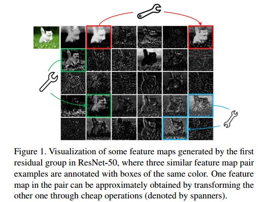
常规的CNN网络提取到的特征图有很多冗余信息，如下图，扳手连接的两个位置的特征图类似。

二、算法原理 

1.Ghost module

常规的卷积公式：，其中  是卷积操作，是输出的特征图，h‘是输出的高，w’是输出的宽，n是输出维度，即卷积核的数量。是卷积核，c是通道数，k是卷积核的高和宽，n是输出维度。

整个卷积操作的FLOPs是：，n和c往往很大。

普通的conv操作如上图a，Ghost module对此进行了改进，第一步是使用更少的卷积核生成输出特征图，如原本的个数是n，现在的个数是m。第二步是对第一步生成的每一张特征图进行cheap operations（depthwise卷积），每张特征图生成s张新特征图（包括一张恒等变换），总共是m×s张，并保证m×s=n，这样保证Ghost module和普通conv输出的特征形状相同。第三步是将这些特征图拼接到一起。

Ghost module的初始卷积公式：，省略了b。其中，m是初始卷积中卷积核的数量，，其余的超参数如卷积核尺寸，步长，padding都是和普通conv一致。

复杂度分析：

(4)式计算的是加速比，分子是普通conv的FLOPS，分母是Ghost module的FLOPS，其中左边是初始卷积的FLOPS，右边是cheap operations的FLOPS。因为分子分母都有相同的因子n*h'*w'，所以可以约掉，又因为d  k，所以将k * k约掉，又因为s << c，最终得到s。

(5)式计算的是压缩比，分子是普通conv卷积核的大小，分母是Ghost module的大小，其中左边是初始卷积卷积核的大小，右边是cheap operations的大小，最终也是得到s。

代码分析：

class GhostModule(nn.Module):
    def __init__(self, inp, oup, kernel_size=1, ratio=2, dw_size=3, stride=1, relu=True):
        super(GhostModule, self).__init__()
        self.oup = oup
        init_channels = math.ceil(oup / ratio)
        new_channels = init_channels*(ratio-1)

        self.primary_conv = nn.Sequential(
            nn.Conv2d(inp, init_channels, kernel_size, stride, kernel_size//2, bias=False),
            nn.BatchNorm2d(init_channels),
            nn.ReLU(inplace=True) if relu else nn.Sequential(),
        )

        self.cheap_operation = nn.Sequential(
            nn.Conv2d(init_channels, new_channels, dw_size, 1, dw_size//2, groups=init_channels, bias=False),
            nn.BatchNorm2d(new_channels),
            nn.ReLU(inplace=True) if relu else nn.Sequential(),
        )

    def forward(self, x):
        x1 = self.primary_conv(x)
        x2 = self.cheap_operation(x1)
        out = torch.cat([x1,x2], dim=1)
        return out[:,:self.oup,:,:]

2.Ghost Bottlenecks

Ghost Bottleneck主要由两个Ghost module堆叠而成，第一个Ghost module用于增加通道数，第二个Ghost module用于减少通道数，然后shortcut用于连接两个Ghost module的输入和输出。每一个Ghost module后都会接一个BN和Relu操作，但是受MobileNetV2的启发，第二个Ghost module后没有Relu。当stride=2时，会在两个Ghost module之间插入一个降采样层和一个步长为2的depthwise convolution操作。

代码分析：

def depthwise_conv(inp, oup, kernel_size=3, stride=1, relu=False):
    return nn.Sequential(
        nn.Conv2d(inp, oup, kernel_size, stride, kernel_size//2, groups=inp, bias=False),
        nn.BatchNorm2d(oup),
        nn.ReLU(inplace=True) if relu else nn.Sequential(),
    )

class SELayer(nn.Module):
    def __init__(self, channel, reduction=4):
        super(SELayer, self).__init__()
        self.avg_pool = nn.AdaptiveAvgPool2d(1)
        self.fc = nn.Sequential(
                nn.Linear(channel, channel // reduction),
                nn.ReLU(inplace=True),
                nn.Linear(channel // reduction, channel),        )

    def forward(self, x):
        b, c, _, _ = x.size()
        y = self.avg_pool(x).view(b, c)
        y = self.fc(y).view(b, c, 1, 1)
        y = torch.clamp(y, 0, 1)
        return x * y

class GhostBottleneck(nn.Module):
    def __init__(self, inp, hidden_dim, oup, kernel_size, stride, use_se):
        super(GhostBottleneck, self).__init__()
        assert stride in [1, 2]

        self.conv = nn.Sequential(
            # pw
            GhostModule(inp, hidden_dim, kernel_size=1, relu=True),
            # dw
            depthwise_conv(hidden_dim, hidden_dim, kernel_size, stride, relu=False) if stride==2 else nn.Sequential(),
            # Squeeze-and-Excite
            SELayer(hidden_dim) if use_se else nn.Sequential(),
            # pw-linear
            GhostModule(hidden_dim, oup, kernel_size=1, relu=False),
        )

        if stride == 1 and inp == oup:
            self.shortcut = nn.Sequential()
        else:
            self.shortcut = nn.Sequential(
                depthwise_conv(inp, inp, 3, stride, relu=True),
                nn.Conv2d(inp, oup, 1, 1, 0, bias=False),
                nn.BatchNorm2d(oup),
            )

    def forward(self, x):
        return self.conv(x) + self.shortcut(x)

3.GhostNet

上面的网络结构是仿照MobileNetV3搭建的，只是一种可能的搭建方法。

代码分析：

class GhostNet(nn.Module):
    def __init__(self, cfgs, num_classes=1000, width_mult=1.):
        super(GhostNet, self).__init__()
        # setting of inverted residual blocks
        self.cfgs = cfgs

        # building first layer
        output_channel = _make_divisible(16 * width_mult, 4)
        layers = [nn.Sequential(
            nn.Conv2d(3, output_channel, 3, 2, 1, bias=False),
            nn.BatchNorm2d(output_channel),
            nn.ReLU(inplace=True)
        )]
        input_channel = output_channel

        # building inverted residual blocks
        block = GhostBottleneck
        for k, exp_size, c, use_se, s in self.cfgs:
            output_channel = _make_divisible(c * width_mult, 4)
            hidden_channel = _make_divisible(exp_size * width_mult, 4)
            layers.append(block(input_channel, hidden_channel, output_channel, k, s, use_se))
            input_channel = output_channel
        self.features = nn.Sequential(*layers)

        # building last several layers
        output_channel = _make_divisible(exp_size * width_mult, 4)
        self.squeeze = nn.Sequential(
            nn.Conv2d(input_channel, output_channel, 1, 1, 0, bias=False),
            nn.BatchNorm2d(output_channel),
            nn.ReLU(inplace=True),
            nn.AdaptiveAvgPool2d((1, 1)),
        )
        input_channel = output_channel

        output_channel = 1280
        self.classifier = nn.Sequential(
            nn.Linear(input_channel, output_channel, bias=False),
            nn.BatchNorm1d(output_channel),
            nn.ReLU(inplace=True),
            nn.Dropout(0.2),
            nn.Linear(output_channel, num_classes),
        )

        self._initialize_weights()

    def forward(self, x):
        x = self.features(x)
        x = self.squeeze(x)
        x = x.view(x.size(0), -1)
        x = self.classifier(x)
        return x

    def _initialize_weights(self):
        for m in self.modules():
            if isinstance(m, nn.Conv2d):
                nn.init.kaiming_normal_(m.weight, mode='fan_out', nonlinearity='relu')
            elif isinstance(m, nn.BatchNorm2d):
                m.weight.data.fill_(1)
                m.bias.data.zero_()


def ghost_net(**kwargs):
    """
    Constructs a MobileNetV3-Large model
    """
    cfgs = [
        # k, t, c, SE, s 
        [3,  16,  16, 0, 1],
        [3,  48,  24, 0, 2],
        [3,  72,  24, 0, 1],
        [5,  72,  40, 1, 2],
        [5, 120,  40, 1, 1],
        [3, 240,  80, 0, 2],
        [3, 200,  80, 0, 1],
        [3, 184,  80, 0, 1],
        [3, 184,  80, 0, 1],
        [3, 480, 112, 1, 1],
        [3, 672, 112, 1, 1],
        [5, 672, 160, 1, 2],
        [5, 960, 160, 0, 1],
        [5, 960, 160, 1, 1],
        [5, 960, 160, 0, 1],
        [5, 960, 160, 1, 1]
    ]
    return GhostNet(cfgs, **kwargs)


if __name__=='__main__':
    model = ghost_net()
    model.eval()
    print(model)
    input = torch.randn(32,3,224,224)
    y = model(input)
    print(y)

三、实验结果

1.特征提取

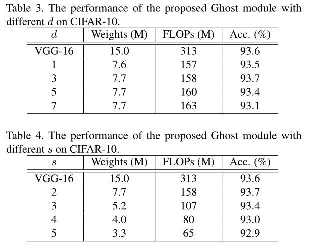
表3是s=2的情况下，不同d和VGG-16的对比，可以看出当d=3时表现最好，这是因为d=1并不能很好的提取到空间信息，d>3会引入过拟合和过多的计算量。

表4是d=3的情况下，不同s和VGG-16的对比，s是直接和计算量相关的参数，因此s越大，计算量越小，压缩比例越大，同时准确率也会下降。当s=2时，模型大小和计算量只有VGG-16的一半了，甚至准确率比它还高，所以选择s=2。

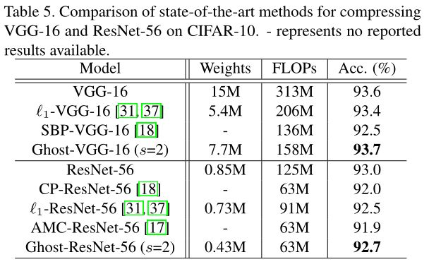
表5中Ghost-VGG-16和Ghost-ResNet-56分别是将VGG-16和ResNet-56中所有的conv操作替换成Ghost module得到的网络，可以看出这两个网络都实现了2x的加速，并且准确率上基本没有损失。

图4和图5同样还是在说明VGG-16提取到的特征图有很多信息冗余，但是Ghost-VGG-16没有，并且提取到的特征图信息与VGG-16差别不大。

表6是GhostNet在ImageNet上测试得到的结果，同样是实现了2x的加速，并且准确率上基本没有损失。

2.图像分类

3.目标检测