MATLAB--数学建模作图大全及代码说明
目录
1、二维曲线
2、二维渐变图
3、二维散点图
4、条形图
5、填充图
6、多Y轴图
7、三维曲线图
8、三维散点图
9、三维伪彩图
10、裁剪伪彩图
11、等高线图
12、三维等高线图
13、等高线填充图
14、三维矢量场图
15、伪彩图+投影图
16、热图
17、分子模型图
18、分形图
1、二维曲线
二维曲线算是最最常见的一种曲线了,它能反应两个变量的因果关系。
clear;
clc;
close all;
x=linspace(1,200,100); %均匀生成数字1-200,共计100个
y1=log(x)+1;  %生成函数y=log(x)+1
y2=log(x)+2;  %生成函数y=log(x)+2
figure;
plot(x,y1); %作图 y=log(x)+1
hold on
plot(x,y2,'LineWidth',2); %作图 y=log(x)+2,LineWidth指线性的宽度,粗细尺寸2
hold off %关闭多图共存在一个窗口上
legend('y1','y2'); %生成图例y1和y2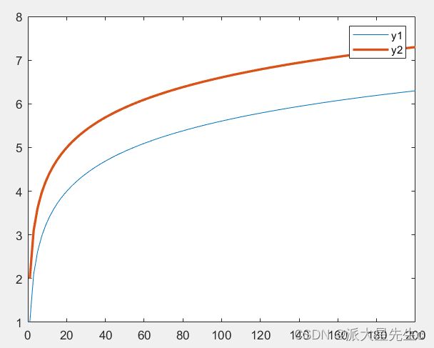
2、二维渐变图
用不同的颜色、数据点大小表征不同数值,更加直观。
x=linspace(0,3*pi,200);
y=cos(x)+rand(1,200); %随机生成1*200,位于[0,1]的数字
sz=25;%尺寸为25
c=linspace(1,10,length(x));
scatter(x,y,sz,c,'filled')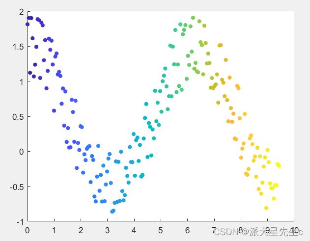
3、二维散点图
常用来比较理论数据和实验数据的趋势关系。
figure;
x=linspace(1,200,100)
y1=log(x)+1;
y3=y1+rand(1,100)-0.5;
plot(x,y1,'LineWidth',2,'Color',[0.21,0.21,0.67]);
hold on;
%设置数据点的型状、数据点的填充颜色、数据点的轮廓颜色
plot(x,y3,'o','LineWidth',2,'Color',[0.46,0.63,0.90],'MarkerFaceColor',[0.35,0.90,0.89],'MarkerEdgeColor',[0.18,0.62,0.17]);
hold off;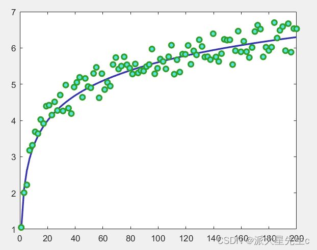
4、条形图
A=[60.689;87.714;143.1;267.9515];
C=[127.5;160.4;231.9;400.2];
B=C-A;
D=[A,B,C];
bar1=bar([2:5:17],A,'BarWidth',0.2,'FaceColor','k');
hold on;
bar2=bar([3:5:18],B,'BarWidth',0.2,'FaceColor',[0.5 0.5 0.5]);
hold on;
bar3=bar([4:5:19],C,'BarWidth',0.2,'FaceColor','w');
ylabel('耗时/s');
xlabel('GMM阶数');
legend('训练耗时','测试耗时','总耗时');
labelID={'8阶','16阶','32阶','64阶'};
set(gca,'XTick',3:5:20);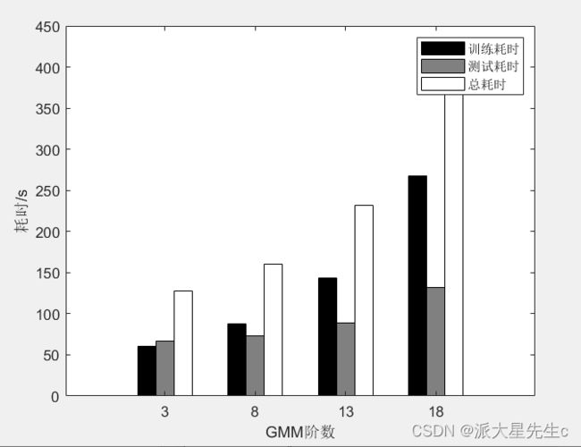
5、填充图
x=0.4:0.1:2*pi;
y1=sin(2*x);
y2=sin(x);
%确定有y1和y2的上下边界
maxY=max([y1;y2]);
minY=min([y1;y2]);
%确定填充多边形,按照顺时针方向来确定点
%fliplr实现左右翻转
xFill=[x,fliplr(x)];
yFill=[maxY,fliplr(minY)];
figure;
fill(xFill,yFill,[0.21,0.21,0.67]);
hold on;
%描绘轮廓线
plot(x,y1,'k','LineWidth',2);
plot(x,y2,'k','LineWidth',2);
hold off;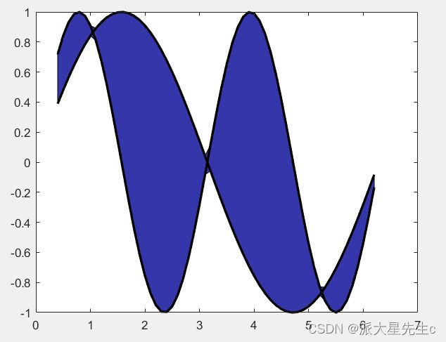
6、多Y轴图
figure;
load('accidents.mat','hwydata');
ind=1:51;
drivers=hwydata(:,5);
yyaxis left;
scatter(ind,drivers,'LineWidth',2);
title('Highway Data');
xlabel('States');
ylabel('Licensed Drivers(thousands)');
pop=hwydata(:,7);
yyaxis right;
scatter(ind,pop,'LineWidth',2);
ylabel('Vehicle Miles Traveled(millions)');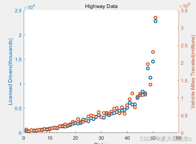
7、三维曲线图
figure;
t=0:pi/20:10*pi;
xt=sin(t);
yt=cos(t);
plot3(xt,yt,t,'-o','Color','b','MarkerSize',10);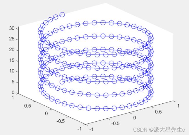
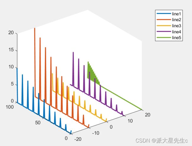
figure;
x=-20:10:20;
y=0:100;
%随便生成的五组数据,也就是目标图上的5条曲线数据
z=zeros(5,101);
z(1,1:10:end)=linspace(1,10,11);
z(2,1:10:end)=linspace(1,20,11);
z(3,1:10:end)=linspace(1,5,11);
z(4,5:10:end)=linspace(1,10,10);
z(5,80:2:end)=linspace(1,5,11);
for i=1:5
    %x方向每条曲线都是一个值,重复y的长度这么多次
    xx=x(i)*ones(1,101);
    %z方向的值,每次取一条
    zz=z(i,:);
    %plot3在xyz空间绘制曲线,保证xyz的长度一致即可
    plot3(xx,y,zz,'LineWidth',2);
    hold on
end
hold off;
legend('line1','line2','line3','line4','line5');
8、三维散点图
figure;
[X,Y,Z]=sphere(16);
x=[0.5*X(:);0.75*X(:);X(:)];
y=[0.5*Y(:);0.75*Y(:);Y(:)];
z=[0.5*Z(:);0.75*Z(:);Z(:)];
S=repmat([70,50,20],numel(X),1);
C=repmat([1,2,3],numel(X),1);
s=S(:);
c=C(:);
h=scatter3(x,y,z,s,c);
h.MarkerFaceColor=[0 0.5 0.5];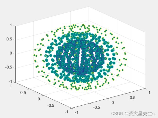
9、三维伪彩图
[x,y,z]=peaks(30);
figure;
plot1=subplot(1,2,1);
surf(x,y,z);
%获取第一幅图的colormap,默认为parula
plot2=subplot(1,2,2);
surf(x,y,z);
%下面设置的是第二幅图的颜色
colormap(hot);
%设置第一幅图颜色显示为parula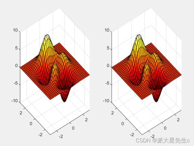
10、裁剪伪彩图
figure;
n=300;
[x,y,z]=peaks(n);
subplot(2,2 ,[1,3]);
surf(x,y,z) ;
shading interp;
view(0,90);
for i=1:n
    for j=1:n
        if x(i,j)^2+2*y(i,j)^2>6&&2*x(i,j)^2+y(i,j)^2<6
            z (i,j)=NaN;
        end
    end
end
subplot(2,2,2);
surf(x,y,z);
shading interp;
view(0,90);
subplot (2,2,4);
surf(x,y,z);
shading interp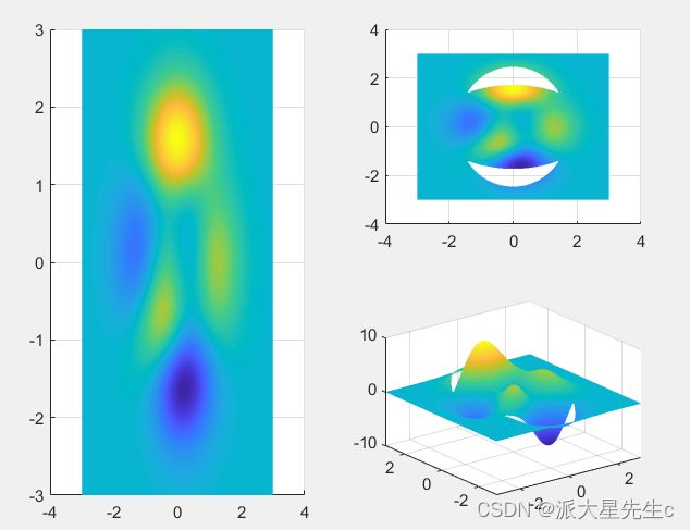
11、等高线图
figure;
[X,Y,Z]=peaks;
subplot(2,2,1);
contour(X,Y,Z,20,'LineWidth',2);
subplot(2,2,2);
contour(X,Y,Z,'--','LineWidth', 2);
subplot(2,2,3);
v=[1,1];
contour(X,Y,Z,v,'LineWidth',2);
x = -2:0.2:2 ;
y = -2 :0.2:3 ;
[X,Y]=meshgrid(x,y);
Z=X.*exp(-X.^2 -Y.^2 );
subplot(2,2,4);
contour(X,Y,Z,'ShowText','on','LineWidth',2);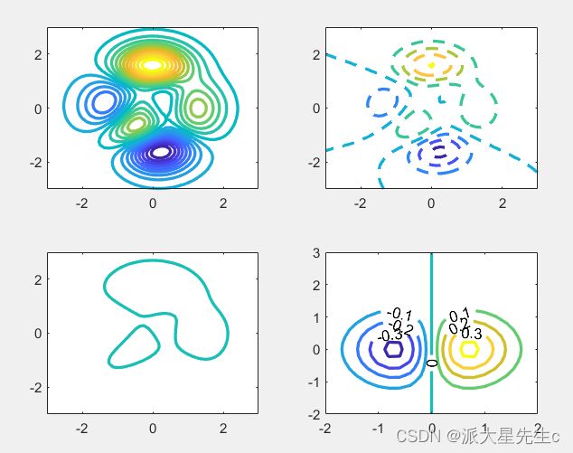
12、三维等高线图
figure('Position',[0,0,900,400]);
subplot(1,3,1);
[X,Y,Z]=sphere(50);
contour3(X,Y,Z,'LineWidth',2);
[X,Y]=meshgrid(-2:0.25:2);
Z=X.*exp(-X.^2-Y.^2);
subplot(1,3,2);
contour3(X,Y,Z,[-0.2 -0.1 0.1 0.2],'ShowText','on','LineWidth',2);
[X,Y,Z]=peaks;
subplot(1,3,3);
contour3(X,Y,Z,[2 2],'LineWidth',2);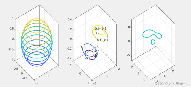
13、等高线填充图
figure;
subplot(2,2,1);
[X,Y,Z]=peaks(5);
contour(X,Y,Z);
subplot(2,2,2);
contourf(X,Y,Z,'--');
%限定范围
subplot(2,2,3);
contourf(X,Y,Z,[2 3],'ShowText','on');
subplot(2,2,4);
contourf(X,Y,Z,[2 2]);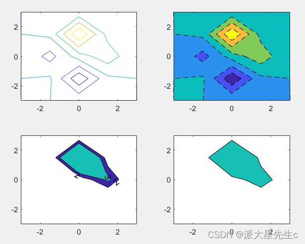
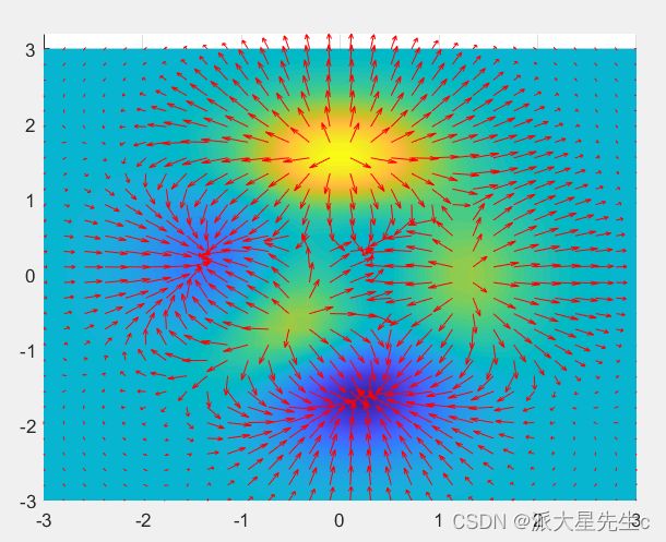
14、三维矢量场图
figure;
[X,Y,Z]=peaks(30);
%矢量场,曲面法线
[U,V,W]=surfnorm(X,Y,Z);
%箭头长度、颜色
quiver3(X,Y,Z,U,V,W,0.5,'r');
hold on;
surf(X,Y,Z);
xlim([-3,3]);
ylim([-3,3.2]);
shading interp;
hold off;
view(0,90);
15、伪彩图+投影图
clear;clc;close all;
x=linspace(-3,3,30);
y=linspace(-4,4,40);
[X,Y]=meshgrid(x,y);
Z=peaks(X,Y);
Z(5:10,15:20)=0;
z1=max(Z);
z2=max(Z,[],2);
figure;
subplot(3,3,[1,2]);
plot(x,z1,'LineWidth',2);
subplot(3 ,3 ,[6,9]);
plot(z2,y,'LineWidth',2);
subplot(3,3,[4,5,7,8]);
surf(x,y,Z);
xlim([-3,3]);
ylim([-4,4]);
view(0,90);
shading interp; %平滑图像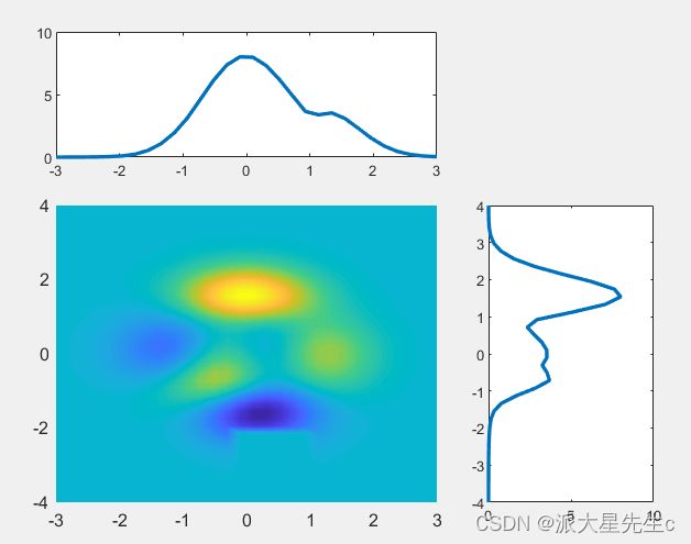
16、热图
clear;
clc;
z=rand(50);
z(z>=0.0&z<0.6)=0.5;
z(z>=0.6&z<0.8)=0.7;
z(z>=0.8&z<=1)=0.9;
for i=1:30
    z(randi(50,1,1):end,i)=nan;
end

for i=31:50
    z(30+randi(20,1,1):end,i)=nan;
end
z(20:25,40:45)=nan;
figure;
%ax=surf(z);
ax=pcolor(z);
view(0,90);
ax.EdgeColor=[1 1 1];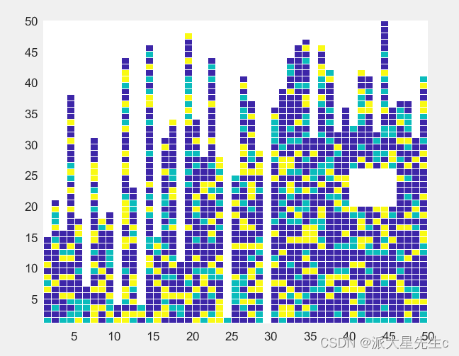
17、分子模型图
clear;
clc;
%球面的坐标信息,为了看起来平滑一点,给到100
[x,y,z]=sphere(100);
%C大小
C=10;
%H大小
H=5;
figure;
%大球
surf(C*x,C*y,C*z,'FaceColor','red','EdgeColor','none');
hold on;
%四个小球,都偏离一点位置,准确的位置需要计算,这里演示一个大概位置
surf(H*x ,H*y,H*z+10,'FaceColor','blue','EdgeColor','none') ;
surf(H*x+10,H*y,H*z-3,'FaceColor','blue','EdgeColor','none');
surf(H*x-4,H*y-10,H*z-3,'FaceColor','blue','EdgeColor','none');
surf(H*x-4,H*y+10,H*z-3,'FaceColor','blue','EdgeColor','none');
%坐标轴设置
axis equal off;
%光源,看起来更有立体感
light
%lighting none,关闭光照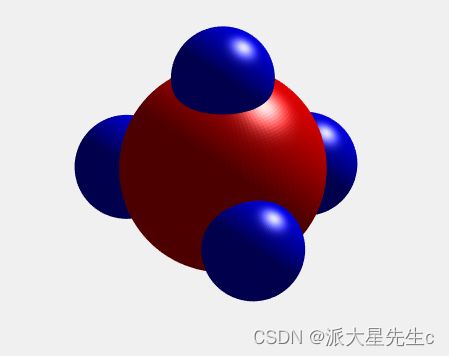
18、分形图
clear;
%不同的参数有不同的图形
a=1.7;
b=1.7;
c=0.6;
d=1.2;
%a=1.5;b=-1.8;c=1.6;d=0.9;
x=0;y=0;
n=100000;
kx=zeros(1,n);
ky=zeros(1,n);
%迭代循环
for i=1:n
    tempx=sin(a*y)+c*cos(a*x);
    tempy=sin(b*x)+d*cos(b*y);
    %存入数组
    kx(i)=tempx;
    ky(i)=tempy;
%重新赋值x,y
x=tempx;
y=tempy;
end
scatter(kx,ky,0.1,'green');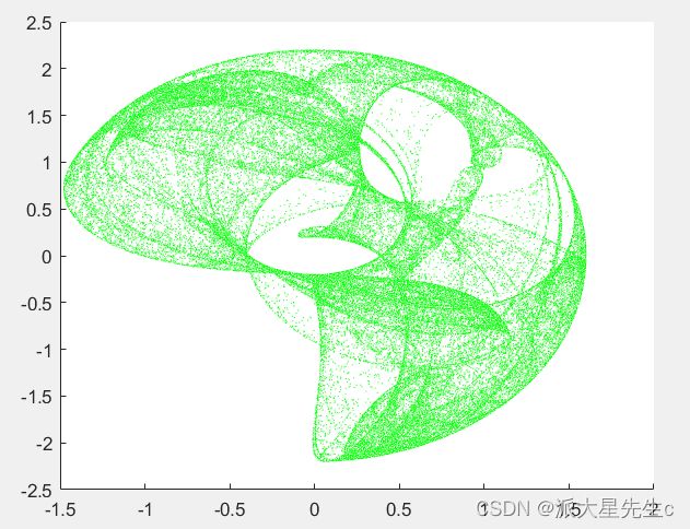
scatter函数用法
●scatter( x ,y )在向量 x和y指定的位置创建一个包含圆形标记的散点图。
●要绘制一组坐标,请将 x和y指定为等长向量。
●要在同一组坐标区上绘制多组坐标,请将 x或 y中的至少一个指定为矩阵。
●s c a tt e r( x ,y ,s z )指定圆大小。要对所有圆使用相同的大小,请将sz指定为标量。要绘制不同大小的每个圆,请将 s z指定为向量或矩阵。
●scatter(x,y,sz,c)指定圆颜色。您可以为所有圆指定一种颜色,也可以更改颜色。例如,您可以通过将c指定为'red '来绘制所有红色圆。
●scatter( _ _ _ ,'f ille d ')填充圆。可以将'fille d '选项与前面语法中的任何输入参数组合一起使用。