多元时间序列预测之LSTM的实现
多元时间序列预测之LSTM的实现
- keras简单介绍
- 多变量LSTM预测模型
本文使用keras库实现基于LSTM的多元时间序列预测问题。所谓多元时间序列预测,是指根据多个变量之间的关系预测他们下一时刻的值。
本文仅搭建LSTM模型进行预测,数据的预处理部分自行完成。
keras简单介绍
keras是一个极简的、高度模块化的神经网络库,可以运行在tensorflow上,具体可看keras中文文档。
具体安装可在网上搜索,非常简单。
多变量LSTM预测模型
1.导入所需的包
from math import sqrt
from numpy import concatenate
from matplotlib import pyplot
import pandas as pd

from sklearn.preprocessing import MinMaxScaler
from sklearn.preprocessing import LabelEncoder
from sklearn.metrics import mean_squared_error
from tensorflow.keras import Sequential

from tensorflow.keras.layers import Dense
from tensorflow.keras.layers import LSTM
from tensorflow.keras.layers import Dropout
from sklearn.model_selection import train_test_split
import matplotlib.pyplot as plt
2.写一个滑动取数据的函数(网上找的)
def time_series_to_supervised(data, n_in=1, n_out=1,dropnan=True):
    """
    :param data:作为列表或2D NumPy数组的观察序列。需要。
    :param n_in:作为输入的滞后观察数(X)。值可以在[1..len(数据)]之间可选。默认为1。
    :param n_out:作为输出的观测数量(y)。值可以在[0..len(数据)]之间。可选的。默认为1。
    :param dropnan:Boolean是否删除具有NaN值的行。可选的。默认为True。
    :return:
    """
    n_vars = 1 if type(data) is list else data.shape[1]
    df = pd.DataFrame(data)
    origNames = df.columns
    cols, names = list(), list()
    cols.append(df.shift(0))
    names += [('%s' % origNames[j]) for j in range(n_vars)]
    n_in = max(0, n_in)
    for i in range(n_in, 0, -1):
        time = '(t-%d)' % i
        cols.append(df.shift(i))
        names += [('%s%s' % (origNames[j], time)) for j in range(n_vars)]
    n_out = max(n_out, 0)
    for i in range(1, n_out+1):
        time = '(t+%d)' % i
        cols.append(df.shift(-i))
        names += [('%s%s' % (origNames[j], time)) for j in range(n_vars)]
    agg = pd.concat(cols, axis=1)
    agg.columns = names
    if dropnan:
        agg.dropna(inplace=True)
    return agg
这个函数,给定输入、输出序列的长度,它可以自动地将时间序列数据转型为适用于监督学习的数据, 它可以将单变量或多变量的时间序列数据帧转化为适用于监督学习的数据帧。
它包含4个参数:
- data: 观测序列。格式是一个 list 或 2维 Numpy Array required
- n_in: 观测数据input(X)的步长,范围[1, len(data)], 默认为1
- n_out: 观测数据output(y)的步长, 范围为[0, len(data)-1], 默认为1
- dropnan: 是否删除存在NaN的行,默认为True
它的返回值只有一个, 即转型后适用于监督学习的 DataFrame
新的DataFrame每一列名字都可被变量编号与时间步长适当的命名,我们就可以用它来进行不同时间步长的时间序列预测了
3.加载数据
这里放一下我的数据:
链接:链接:https://pan.baidu.com/s/13Y57gKqtfpmq7-7T1B73Iw
提取码:6tbb
# 加载数据
path1 = r"C:\data.xlsx"#数据所在路径
#我的数据是excel表,若是csv文件用pandas的read_csv()函数替换即可。
datas1 = pd.DataFrame(pd.read_excel(path1))
#我只取了data表里的第3、23、16、17、18、19、20、21、27列,如果取全部列的话这一行可以去掉
data1 = datas1.iloc[:,np.r_[3,23,16:22,27]]
data1=data1.interpolate()
values1 = data1.values
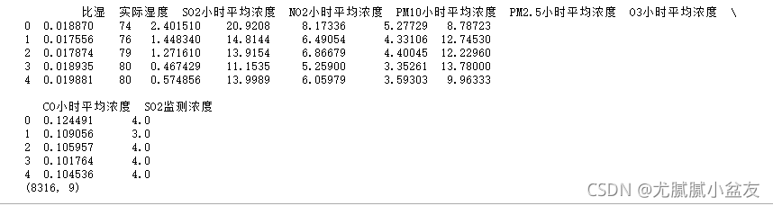
print(data1.head())
print(data1.shape)
打印一下data1的head和shape,可以确认一下是不是要处理的数据
4.归一化处理,去除量纲差别
#首先归一化,再移位处理,得到训练样本
scaler = MinMaxScaler(feature_range=(0, 1))
scaledData1 = scaler.fit_transform(data1)
print(scaledData1.shape)
5.使用time_series_to_supervised函数生成适用于监督学习的 DataFrame
n_steps_in =72 #历史时间长度
n_steps_out=1#预测时间长度
processedData1 = time_series_to_supervised(scaledData1,n_steps_in,n_steps_out)
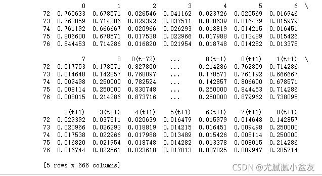
print(processedData1.head())
可以打印一下看看生成的dataframe:
6.划分特征与标签
data_x = processedData1.loc[:,'0(t-72)':'8(t-1)']
data_y = processedData1.loc[:,'0':'8']
如果你只是预测9个特征中的其中1个或几个特征的值,在data_y这里做相应调整。比如,我只想预测“So2监测浓度”(第九列)的数据,那第二行应改为:
data_y = processedData1.loc[:,'8']
值得注意的是:若我们对data_y进行修改,比如我们仅预测特征最后一列时,后面对模型预测结果进行反归一化会报出维数不匹配的问题。这是因为我们一开始归一化fit_transform()的是整个数据集,包含了所有的特征列,而后续我们想反归一化时,仅是对我们想要预测的值,即单一特征列,进行反归一化,所以会出现维数不匹配的情况。建议可以预测所有特征列,最后结果仅提取你想要的预测列结果即可,像我下面仅使用了预测结果的最后一列,即y_pre[:,8]一样。或者sklearn.preprocessing.MinMaxScaler.inverse_transform()是否可以仅对部分列反归一化,从而消除维数不匹配问题(我在网上没有搜到相关用法,有知道的可以在评论区补充哦~)
7.划分训练集和测试集
train_X1,test_X1, train_y, test_y = train_test_split(data_x.values, data_y.values, test_size=0.4, random_state=343)
# reshape input to be 3D [samples, timesteps, features]
train_X = train_X1.reshape((train_X1.shape[0], n_steps_in, scaledData1.shape[1]))
test_X = test_X1.reshape((test_X1.shape[0], n_steps_in, scaledData1.shape[1]))
print(train_X.shape, train_y.shape, test_X.shape, test_y.shape)
使用train_test_split函数划分训练集和测试集,测试集的比重是40%。
然后将train_X1、test_X1进行一个升维,变成三维,维数分别是[samples,timesteps,features]。打印一下他们的shape:
![]()
8.构建模型
# design network
model = Sequential()
#input_shape千万不要写错!,第一个参数可以更改
model.add(LSTM(96,return_sequences=True, input_shape=(train_X.shape[1], train_X.shape[2])))
model.add(Dropout(0.2))
model.add(LSTM(64, return_sequences=False)) # returns a sequence of vectors of dimension 32
model.add(Dropout(0.2))
model.add(Dense(32))
model.add(Dropout(0.2))
model.add(Dense(train_y.shape[1]))
model.compile(loss='mse', optimizer='adam')
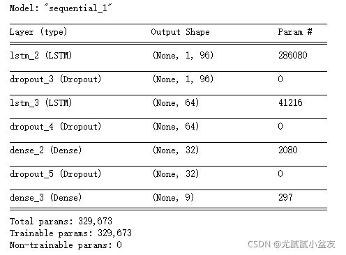
print(model.summary())
# fit network
history = model.fit(train_X, train_y, epochs=30, batch_size=64, validation_data=(test_X, test_y), verbose=2,
shuffle=False)
# plot history
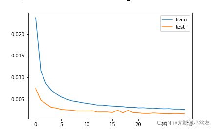
plt.plot(history.history['loss'], label='train')
plt.plot(history.history['val_loss'], label='test')
plt.legend()
plt.show()
这个地方model.add中间随便加,Dense是全连接层,dropout是随机减少网络中链接的神经元数。
但是,第一行的input_shape地方不要随意改变,最后一行的“model.add(Dense(train_y.shape[1]))”也不要改!最后一行的Dense里面的值要和你的期望输出一致,也就是,如果你想预测的是9个特征,里面就填9,如果是预测一个特征,就填1,和上面data_y的特征维度相同。
输出结果:
loss变化图:
9.使用模型
 # 预测
yhat = model.predict(test_X)
# 反归一化
inv_forecast_y = scaler.inverse_transform(yhat)
inv_test_y = scaler.inverse_transform(test_y)
用predict方法进行预测。因为之前我们对数据进行了归一化处理,所以要想获得真实的预测值,需要反归一化。
9.计算均方误差与画图
# 计算均方根误差
rmse = sqrt(mean_squared_error(inv_test_y[:,8], inv_forecast_y[:,8]))
print('Test RMSE: %.3f' % rmse)
#画图
plt.figure(figsize=(16,8))
plt.plot(inv_test_y[:,8], label='true')
plt.plot(inv_forecast_y[:,8], label='pre')
plt.legend()
plt.show()
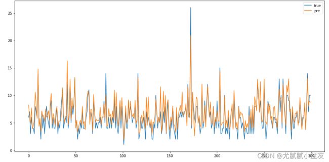
这里我只做了对第九列“So2监测浓度”的预测值与实际值的均方误差与图像对比,因为数据太多,只展示了前300行的数据。从图片看拟合程度还是不错的。
请注意,图片展示的是测试集中的部分数据,因为我们一开始将训练集和测试集打乱顺序划分的,所以下图展示数据并非时序。如果想要获得时序数据,有两种方法:1.划分训练集和测试集的时候不打乱顺序,按顺序划分,比如前80%为训练集,后20%为测试集;2.使用data_x输入模型获得的预测值与data_y比较(注意data_x输入模型时需要升维),这个数据可以用来画图展示,但不能用来得到模型的rmse或mse等评价值,因为包含训练集的数据,会放大模型的效果。
以上模型就训练好可以使用了。
10.使用模型
#预测数据
#预测数据
data_x1= data_x.values[-1:,:]
print(data_x.shape)
data_x1= data_x1.reshape((data_x1.shape[0], n_steps_in, scaledData1.shape[1]))

yhat_pre= model.predict(data_x1)

# 逆转预测值
yhat_pre= scaler.inverse_transform(yhat_pre)
print(yhat_pre)
使用表中给出的数据预测下一时刻的9个特征的值,结果如下:
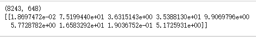
这里一定要记得data_x1需要升维才能喂给LSTM!还有,我这里使用的data_x是已经经过前面time_series_to_supervised函数处理过的,如果你换了个新的数据,记得要先处理一下,把它变成这种步长内的数据横向拼接的形式。
全部代码:
from math import sqrt
from numpy import concatenate
from matplotlib import pyplot
import pandas as pd
# from pandas import read_csv
# from pandas import DataFrame
# from pandas import concat
from sklearn.preprocessing import MinMaxScaler
from sklearn.preprocessing import LabelEncoder
from sklearn.metrics import mean_squared_error
from tensorflow.keras import Sequential
# from keras import models
from tensorflow.keras.layers import Dense
from tensorflow.keras.layers import LSTM
from tensorflow.keras.layers import Dropout
from sklearn.model_selection import train_test_split
import matplotlib.pyplot as plt
import numpy as np

def time_series_to_supervised(data, n_in=1, n_out=1,dropnan=True):
    """
    :param data:作为列表或2D NumPy数组的观察序列。需要。
    :param n_in:作为输入的滞后观察数(X)。值可以在[1..len(数据)]之间可选。默认为1。
    :param n_out:作为输出的观测数量(y)。值可以在[0..len(数据)]之间。可选的。默认为1。
    :param dropnan:Boolean是否删除具有NaN值的行。可选的。默认为True。
    :return:
    """
    n_vars = 1 if type(data) is list else data.shape[1]
    df = pd.DataFrame(data)
    origNames = df.columns
    cols, names = list(), list()
    cols.append(df.shift(0))
    names += [('%s' % origNames[j]) for j in range(n_vars)]
    n_in = max(0, n_in)
    for i in range(n_in, 0, -1):
        time = '(t-%d)' % i
        cols.append(df.shift(i))
        names += [('%s%s' % (origNames[j], time)) for j in range(n_vars)]
    n_out = max(n_out, 0)
    for i in range(1, n_out+1):
        time = '(t+%d)' % i
        cols.append(df.shift(-i))
        names += [('%s%s' % (origNames[j], time)) for j in range(n_vars)]
    agg = pd.concat(cols, axis=1)
    agg.columns = names
    if dropnan:
        agg.dropna(inplace=True)
    return agg

# 加载数据
path1 = r"C:\data.xlsx"
datas1 = pd.DataFrame(pd.read_excel(path1))
data1 = datas1.iloc[:,np.r_[3,23,16:22,27]]
data1=data1.interpolate()
values1 = data1.values
#首先归一化,再移位处理,得到训练样本
scaler = MinMaxScaler(feature_range=(0, 1))
scaledData1 = scaler.fit_transform(data1)

n_steps_in =72 #历史时间长度
n_steps_out=1#预测时间长度
processedData1 = time_series_to_supervised(scaledData1,n_steps_in,n_steps_out)
print(processedData1.head())

data_x = processedData1.loc[:,'0(t-72)':'8(t-1)']
data_y = processedData1.loc[:,'0':'8']

train_X1,test_X1, train_y, test_y = train_test_split(data_x.values, data_y.values, test_size=0.4, random_state=343)
# reshape input to be 3D [samples, timesteps, features]
train_X = train_X1.reshape((train_X1.shape[0], n_steps_in, scaledData1.shape[1]))
test_X = test_X1.reshape((test_X1.shape[0], n_steps_in, scaledData1.shape[1]))
print(train_X.shape, train_y.shape, test_X.shape, test_y.shape)


# design network
model = Sequential()
model.add(LSTM(96,return_sequences=True, input_shape=(train_X.shape[1], train_X.shape[2])))
model.add(Dropout(0.2))
model.add(LSTM(64, return_sequences=False))  # returns a sequence of vectors of dimension 32
model.add(Dropout(0.2))
model.add(Dense(32))
model.add(Dropout(0.2))
model.add(Dense(train_y.shape[1]))
model.compile(loss='mse', optimizer='adam')
print(model.summary())
# fit network
history = model.fit(train_X, train_y, epochs=30, batch_size=64, validation_data=(test_X, test_y), verbose=2,
                    shuffle=False)
# plot history
plt.plot(history.history['loss'], label='train')
plt.plot(history.history['val_loss'], label='test')
plt.legend()
plt.show()

 # 预测
yhat = model.predict(test_X)
# 逆转预测值
print(yhat[:,8])
inv_forecast_y = scaler.inverse_transform(yhat)
    # 逆转实际值
inv_test_y = scaler.inverse_transform(test_y)
# 计算均方根误差
rmse = sqrt(mean_squared_error(inv_test_y[:,8], inv_forecast_y[:,8]))
print('Test RMSE: %.3f' % rmse)
#画图
plt.figure(figsize=(16,8))
plt.plot(inv_test_y[0:300,8], label='true')
plt.plot(inv_forecast_y[0:300,8], label='pre')
plt.legend()
plt.show()