调研题目 Image Indentification and Deep Learning——Thinking after Freshman Lecture
电子科技大学 格拉斯哥学院 2017级 叶子鉴
Author Ye Zijian, Glassgow College
Preface
Photo identification may be used for face-to-face authentication of identity of a party who either is personally unknown to the person in authority or because that person does not have access to a file, a directory, a registry or an information service that contains or that can render a photograph of somebody on account of that person’s name and other personal information.
Abstract
The basis of the image indentification is deep learning which is also known as deep structured learning or hierarchical learning) is part of a broader family of machine learning methods based on learning data representations, as opposed to task-specific algorithms. Learning can be supervised, semi-supervised or unsupervised.
Main Body
Section 1
The main point of the machine learning is as below.

Most human solutions do not rely on clear laws and machines models solve problems in their own way, which is more efficient than people’s in some cases.
Section 2

Supervised learning of neural networks (basic steps)
Step 1:Initializing weight coefficients (with appropriate values)
Step 2:Extract a training sample {input, correct output}, input it into NN;Compare and calculate the error between NN output and correct output.
Step 3:Adjust the weight coefficient to reduce the above error.
Step 4:Repeat Step 2-3 until all training samples are traversed.

Supervised learning of neural networks (basic steps)
Section 2
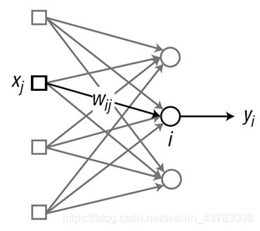
Single layer neural network training – Delta rule
S1:Initializing weight coefficients (with appropriate values)
S2:Extract a training sample {input, correct output}Plug in NN to compute node output and correct output the difference between the:
![]()
S3:According to the delta rule, calculate the weight update amount:

S4:Cumulative value
![]()
S5:Repeat Step 2-4 until all training data is traversed.
S6:Repeat Step 2-5 until the error is acceptable (preset threshold)
Section3
Three commonly used weight update algorithms
Batch Algorithm Code (Matlab)
clear all %to clear the workspace
X = [ 0 0 1;
         0 1 1;
         1 0 1;
         1 1 1];
D = [ 0 0 1 1];
W = 2*rand(1, 3) - 1;
for epoch = 1:40000  %40000 turns training
W = DeltaBatch(W, X, D);
end
for k = 1:4 % calculate the network output after training
  x = X(k, :)';
  v = W*x;
  y = Sigmoid(v)
end
function W = DeltaBatch(W, X, D)
alpha = 0.9; N = 4;
dWsum = zeros(3, 1);
for k = 1:N
x = X(k, :)';
d = D(k);
v = W*x;
y = Sigmoid(v);
e = d - y;
delta = y*(1-y)*e;
dW = alpha*delta*x;
dWsum = dWsum + dW;
end
dWavg = dWsum / N;
W = W + dWavg’;
end
MiniBatch Algorithm Code (Matlab)
clear all

X = [ 0 0 1;

         0 1 1;

         1 0 1;

         1 1 1];

D = [ 0 0 1 1];

W = 2*rand(1, 3) - 1;

for epoch = 1:20000  %

  W = DeltaMiniBatch(W, X, D);

end

for k = 1:4 %

  x = X(k, :)';

  v = W*x;

  y = Sigmoid(v)

end

function W = DeltaMiniBatch(W,
X, D)

    alpha = 0.9; N = 4;  M=2;

    for k = 1 : (N/M)

        dWsum = zeros(3, 1);

        for j = 1 : M

            id = (k-1)*M+j;

            x = X(id, :)';  d = D(id);

            v = W*x;       y = Sigmoid(v);

            e = d - y;

            delta = y*(1-y)*e;

            dW = alpha*delta*x;

            dWsum = dWsum + dW;

      end

      dWavg = dWsum / M;

      W=W+dWavg';

  end

end
Neural networks are networks of nodes that mimic neurons in the human brain.The node calculates the weighted sum of the input signals and puts it into the activation function output
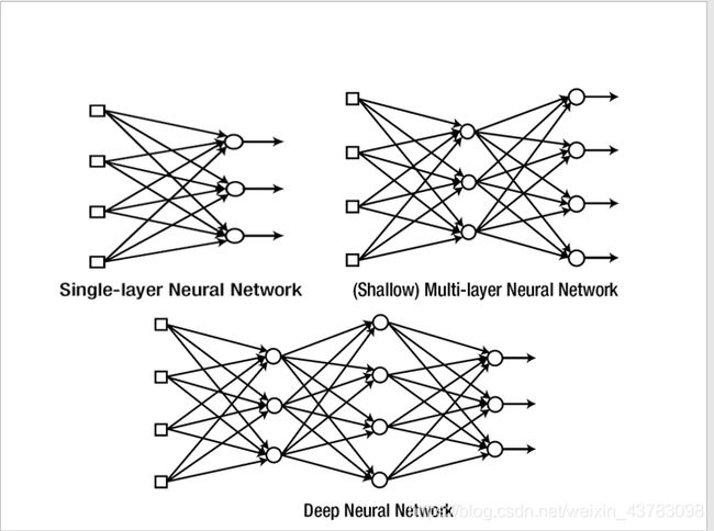
Neural networks are usually constructed in layers: signals flow from the input layer to the hidden layer and then to the output layer.
The linear activation function used in the hidden layer is invalid (reducible), and the output layer can be used.
Monitor learning process: adjust weights to reduce the difference between network output and expected output.
Learning rules: method of adjusting weight coefficient according to training data
Section4
BP algorithm
Backpropagation is a method used in artificial neural networks to calculate a gradient that is needed in the calculation of the weights to be used in the network.Backpropagation is shorthand for “the backward propagation of errors,” since an error is computed at the output and distributed backwards throughout the network’s layers.[2] It is commonly used to train deep neural networks,[3] a term referring to neural networks with more than one hidden layer.[4]
Backpropagation is a special case of a more general technique called automatic differentiation. In the context of learning, backpropagation is commonly used by the gradient descent optimization algorithm to adjust the weight of neurons by calculating the gradient of the loss function.

<—————————Back propagation error—————————
Step1:Initializes the weight coefficient
Step2: A training sample {x,y} was extracted to calculate the output of the neural networkCalculates the difference between the network output and the expected outputAnd delta for the output node.
Step3: Propagate the delta of the output node backward to calculate the delta of the node at the previous layer.
Step4: Repeat Step 3 until you reach the first hidden layer
Step5: Adjust the weight coefficient of each layer
Step6: Repeat Step 2-5 to go through each training sample
Step7: Repeat Step 2-6 until the output error meets the expectation
Example
Training multi-layer neural networks to solve XOR problems
Training data
{0,0,1, 0}
{0,1,1, 1}
{1,0,1, 1}
{1,1,1, 0}
clear all

X = [ 0 0 1; 0 1 1; 1 0 1; 1
1 1]; %Input training data

D = [ 0  1
1  0]; %Output training data

W1 = 2*rand(4, 3) - 1; %Initializes the layer 1 weight matrix

W2 = 2*rand(1, 4) - 1; %Initializes the layer 2 weight matrix

for epoch = 1:10000    % Training 10000 round

       [W1 W2] = BackpropXOR(W1, W2, X, D); %Each round updates the weight of each layer
end

% After the training, put in 4 training data in turn to verify the output results:

for k = 1:4

x  = X(k, :)';

v1 = W1*x;

y1 = Sigmoid(v1);

v  = W2*y1;


y  = Sigmoid(v)

end
Conclusion
Deep learning is closely related to a class of theories of brain development (specifically, neocortical development) proposed by cognitive neuroscientists in the early 1990s.
These developmental theories were instantiated in computational models, making them predecessors of deep learning systems. These developmental models share the property that various proposed learning dynamics in the brain (e.g., a wave of nerve growth factor) support the self-organization somewhat analogous to the neural networks utilized in deep learning models.
Like the neocortex, neural networks employ a hierarchy of layered filters in which each layer considers information from a prior layer (or the operating environment), and then passes its output (and possibly the original input), to other layers.
This process yields a self-organizing stack of transducers, well-tuned to their operating environment. A 1995 description stated, “…the infant’s brain seems to organize itself under the influence of waves of so-called trophic-factors … different regions of the brain become connected sequentially, with one layer of tissue maturing before another and so on until the whole brain is mature.”
Reference
1.Deep learning Wikipedia
https://en.wikipedia.org/wiki/Deep_learning#Criticism_and_comment
2.Photo identification
https://en.wikipedia.org/wiki/Photo_identification
