学习笔记31-自回归-建立时间序列预测模型(ARIMA方法)
时间序列(Time Series)定义: 按照时间的顺序把一个随机事件变化发展的过程记录。
安装包
import pandas as pd
import numpy as np
import matplotlib.pyplot as plt
from datetime import datetime

from matplotlib.pylab import rcParams
rcParams['figure.figsize']=15,6
一、实验数据
数据集包含了两组数据:Cv值-湿度(float型)以及检测的相对时间(object型)。
#1.数据导入和查看,数据集包含了两组数据:CV Time
data=pd.read_csv('test2.csv',nrows=500)#nrows=80,指加载80组数据
#数据导入和查看
print(data.head())
print('\nData Types:')
print(data.dtypes)

#2.数据格式转换,将数据中的时间信息转换成索引。
#格式转换
dateparse=lambda dates: pd.datetime.strptime(dates, '%Y-%m-%d %H:%M:%S')
data=pd.read_csv('test2.csv', parse_dates=['Time'], index_col='Time', date_parser=dateparse, nrows=80)
# parse_dates:指定包含日期时间信息的列。例子里的列名是'Time‘
# index_col:在TS数据中使用pandas的关键是索引必须是日期等时间变量。所以这个参数告诉pandas使用'Time'列作为索引
# date_parser:它指定了一个将输入字符串转换为datetime可变的函数。pandas 默认读取格式为'YYYY-MM-DD HH:MM:SS'的数据。
# 如果这里的时间格式不一样,就要重新定义时间格式,dataparse函数可以用于此目的。
timeseries = data
print(data.head())

二、检验
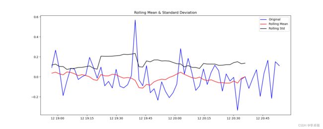
1.平稳性检验
判断依据:如果检验统计量(TS)大于临界值(CV),则否决原假设(即序列不是平稳的)。如果TS小于CV,则不能否决原假设(即序列是平稳的)。
#1.平稳性检验
from statsmodels.tsa.stattools import adfuller
#平稳性检测
def test_stationarity(timeseries):
# Determing rolling statistics
rolmean = timeseries.rolling(10).mean()
rolstd = timeseries.rolling(10).std()
# Plot rolling statistics:
plt.plot(timeseries, color='blue', label='Original')
plt.plot(rolmean, color='red', label='Rolling Mean') # 均值
plt.plot(rolstd, color='black', label='Rolling Std') # 标准差
plt.legend(loc='best')
plt.title('Rolling Mean & Standard Deviation')
plt.savefig("./figure/平稳性检测")
plt.show()
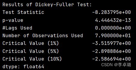
# Perform Dickey-Fuller Test:
print('Results of Dickey-Fuller Test:')
dftest = adfuller(timeseries, autolag='AIC')
dfoutput = pd.Series(dftest[0:4], index=['Test Statistic', 'p-value', '#Lags Used', 'Number of Observations Used'])
for key, value in dftest[4].items():
dfoutput['Critical Value (%s)' % key] = value
print(dfoutput)
test_stationarity(timeseries)


实验结果:在所以的置信区间内,TS
2.KPSS测试
#2.KPSS 测试,不如ADF方法流行。KPSS检验的原假设和备择假设与ADF检验相反。
# define function for ADF
from statsmodels.tsa.stattools import kpss
def kpss_test(timeseries):
    print('Results of KPSS Test:')
    kpsstest = kpss(timeseries, regression='c')
    kpss_output = pd.Series(kpsstest[0:3], index=['Test Statistic', 'p-value', '#Lags Used'])
    for key, value in kpsstest[3].items():
        kpss_output['Critical Value (%s)' % key] = value
    print(kpss_output)
kpss_test(timeseries)  #结果显示TS>cv, p <1% 表示拒绝数据是平稳的原假设,序列不是平稳的。
KPSS检验的原假设和备择假设相反。
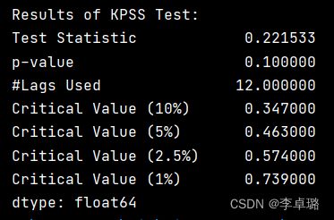
实验结果:在所以的置信区间内,TS
3.消除趋势
#3.消除趋势,结果显示TS>cv, p <1% 表示拒绝数据是平稳的原假设,序列不是平稳的。
ts_log=np.log(timeseries)
# plt.plot(ts_log)
# plt.show()
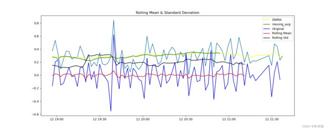
#移动平均,根据时间序列的频率取“k”连续值的平均值。
moving_avg = ts_log.rolling(20).mean() #计算均值
ts_log_moving_avg_diff=ts_log-moving_avg #使用均值的差,使得整体平滑
ts_log_moving_avg_diff.dropna(inplace=True) #丢掉NAN
test_stationarity(ts_log_moving_avg_diff)#查看结果
由fig1可以观察到有明显的噪音。因此,利用对数、开方、开立方的方式惩罚最高项,使得整体平滑。

实验结果:TS
4.EWMA指数加权移动平均
#4.指数加权移动平均(Exponential Weighted Moving Average) 一种流行的方法是指数加权移动平均法,其中权重被分配给所有先前的值,并带有一个衰减因子。
expwighted_avg=pd.DataFrame.ewm(ts_log,halflife=12).mean()
plt.plot(ts_log)
plt.plot(expwighted_avg,color='yellow', label='EWMA')
plt.plot(moving_avg,color='green', label='moving_avg')
ts_log_ewma_diff=ts_log-expwighted_avg
test_stationarity(ts_log_ewma_diff)

实验结果:TS
5.差分
#5.Differencing 差分
ts_log_diff=ts_log-ts_log.shift()

# reduced trend considerably
ts_log_diff.dropna(inplace=True)
test_stationarity(ts_log_diff)

实验结果:TS
三、预测时间序列模型 ARIMA方法
ARIMA(p,d,q)中,AR是“自回归”,p为自回归项数;MA为“滑动平均”,q为滑动平均项数,d为使之成为平稳序列所做的差分次数(阶数)。
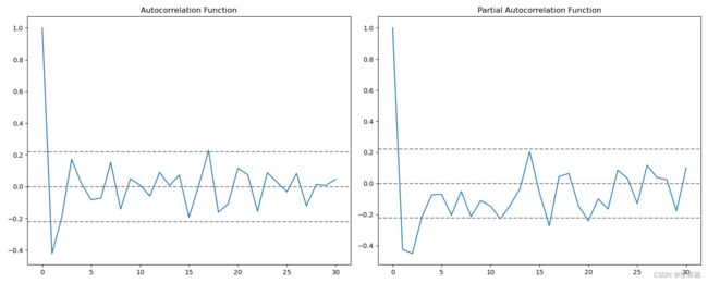
1)ACF;PACF函数
#预测时间序列
from statsmodels.tsa.stattools import acf,pacf
lag_acf=acf(ts_log_diff,nlags=30)
lag_pacf=pacf(ts_log_diff,nlags=30,method='ols')

#1)ACF(Autocorrelation Function),自协方差或自相关函数。
#将有序的随机变量序列与其自身相比较,它反映了同一序列在不同时序的取值之间的相关性。
plt.subplot(121)
plt.plot(lag_acf)
plt.axhline(y=0,linestyle='--',color='gray')
plt.axhline(y=-1.96/np.sqrt(len(ts_log_diff)),linestyle='--',color='gray')
plt.axhline(y=1.96/np.sqrt(len(ts_log_diff)),linestyle='--',color='gray')
plt.title('Autocorrelation Function')


#2)Plot PACF:偏自相关函数(PACF)计算的是严格的两个变量之间的相关性,是剔除了中间变量的干扰之后所得到的两个变量之间的相关程度。
plt.subplot(122)
plt.plot(lag_pacf)
plt.axhline(y=0,linestyle='--',color='gray')
plt.axhline(y=-1.96/np.sqrt(len(ts_log_diff)),linestyle='--',color='gray')
plt.axhline(y=1.96/np.sqrt(len(ts_log_diff)),linestyle='--',color='gray')
plt.title('Partial Autocorrelation Function')
plt.tight_layout()
plt.savefig("./figure/平稳性检测")
plt.show()
Fig5所示。左:ACF(Autocorrelation Function),自协方差或自相关函数。将有序的随机变量序列与其自身相比较,它反映了同一序列在不同时序的取值之间的相关性。直观上来说,ACF 描述了一个观测值和另一个观测值之间的自相关,包括直接和间接的相关性信息。右:PACF:偏自相关函数(PACF)计算的是严格的两个变量之间的相关性,是剔除了中间变量的干扰之后所得到的两个变量之间的相关程度。
其中:p—PACF图第一次穿过置信区间上限的滞后值(0)。q—ACF图第一次穿过置信区间上限的滞后值(0)。
2)AR model 自回归模型
#AR model 自回归模型;是统计上一种处理时间序列的方法,用同一变数例如x的之前各期,亦即x1至xt-1来预测本期xt的表现,并假设它们为一线性关系。
from statsmodels.tsa.arima_model import ARIMA
model = ARIMA(ts_log,order=(2,1,0))
results_AR=model.fit(disp=-1)
result=pd.DataFrame(results_AR.fittedvalues, columns=['CV'])
plt.plot(ts_log_diff,color='blue', label='ts_log')
plt.plot(results_AR.fittedvalues,color='red', label='results_AR')
plt.title('RSS: %.4f'% ((result-ts_log_diff)**2).sum())#RSS是残差值
plt.savefig("./figure/平稳性检测")
plt.show()
AR是统计上一种处理时间序列的方法,用同一变数例如x的之前各期,亦即x1至xt-1来预测本期xt的表现,并假设它们为一线性关系。其中,RSS是残差值=1.95。

3)MA model 移动平均模型
#MA model 移动平均模型关注的是自回归模型中的误差项的累加。它能够有效地消除预测中的随机波动。
model = ARIMA(ts_log,order=(0,1,2))
results_MA=model.fit(disp=-1)
result=pd.DataFrame(results_MA.fittedvalues, columns=['CV'])
plt.plot(ts_log_diff,color='blue', label='ts_log')
plt.plot(results_MA.fittedvalues,color='red', label='results_MA')
plt.title('RSS: %.4f'% ((result-ts_log_diff)**2).sum())
plt.savefig("./figure/平稳性检测")
plt.show()
MA关注的是自回归模型中的误差项的累加。它能够有效地消除预测中的随机波动。RSS=1.6569。

4)组合模型
#组合模型
model = ARIMA(ts_log,order=(2,1,2))
results_ARIMA=model.fit(disp=-1)
result=pd.DataFrame(results_ARIMA.fittedvalues, columns=['CV'])
plt.plot(ts_log_diff,color='blue', label='ts_log')
plt.plot(results_ARIMA.fittedvalues,color='red', label='results_ARIMA')
plt.title('RSS: %.4f'% ((result-ts_log_diff)**2).sum())
plt.savefig("./figure/平稳性检测")
plt.show()
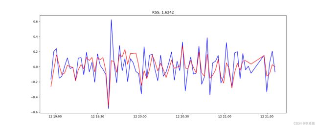
RSS=1.6242。 Fig8发现MA和组合差不多,结果要比AR效果好。