【心电信号】Simulink胎儿心电信号提取【含Matlab源码 1550期】
⛄一、心电信号简介
0 引言
心电信号是人类最早研究的生物信号之一, 相比其他生物信号更易于检测, 且具有直观的规律。心电图的准确分析对心脏病的及早治疗有重大的意义。人体是一个复杂精密的系统, 有许多不可抗的外界因素, 得到纯净的心电信号非常困难。可以采用神经网络算法去除心电信号的噪声, 但这种方法存在训练难度大、耗时长的缺点。小波变换在处理非线性、非平稳且奇异点较多的信号时具有一定的优越性, 近年来许多学者使用其对心电信号进行研究。
1 心电信号简介
心电信号由以下几个波段组成, 一个典型的心电图如图1所示。

图1 典型心电图
(1) P波:反映心房肌在除极过程中的电位变化过程;
(2) P-R间期:反映的是激动从窦房结通过房室交界区到心室肌开始除极的时限;
(3) QRS波群:反映心室肌除极过程的电位变化;
(4) T波:代表心室肌复极过程中所引起的电位变化;
(5) S-T段:从QRS波群终点到达T波起点间的一段水平线[2];
(6) Q-T间期:心室从除极到复极的时间[3];
(7) U波:代表动作电位的后电位。
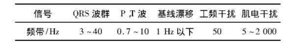
由于心电信号十分微弱, 且低频, 极易受到干扰, 不同的干扰源的噪声虽是随机的, 但来自同一个干扰源的噪声往往具有同一类特征。分析干扰的来源, 针对不同的来源使用合适的处理方法, 是数据采集重点考虑的一个问题。常见干扰有3种: (1) 工频干扰; (2) 基线漂移; (3) 肌电干扰。其中已经证明小波变换在抑制心电信号的工频干扰方面具有较大优势。具体噪声频带如表1所示。
表1 心电信号以及主要噪声频带
⛄二、部分源代码
%% Init
% clear all; close all;
Fs = 4e3;
Time = 40;
NumSamp = Time * Fs;
load Hd;
%% Mom’s Heartbeat
% In this example, we shall simulate the shapes of the electrocardiogram
% for both the mother and fetus. The following commands create an
% electrocardiogram signal that a mother’s heart might produce assuming
% a 4000 Hz sampling rate. The heart rate for this signal is approximately
% 89 beats per minute, and the peak voltage of the signal is 3.5 millivolts.
x1 = 3.5ecg(2700).'; % gen synth ECG signal
y1 = sgolayfilt(kron(ones(1,ceil(NumSamp/2700)+1),x1),0,21); % repeat for NumSamp length and smooth
n = 1:TimeFs’;
del = round(2700*rand(1)); % pick a random offset
mhb = y1(n + del)'; %construct the ecg signal from some offset
axis([0 2 -4 4]);
grid;
xlabel(‘Time [sec]’);
ylabel(‘Voltage [mV]’);
title(‘Maternal Heartbeat Signal’);
%% Fetus Heartbeat
% The heart of a fetus beats noticeably faster than that of its mother,
% with rates ranging from 120 to 160 beats per minute. The amplitude of the
% fetal electrocardiogram is also much weaker than that of the maternal
% electrocardiogram. The following series of commands creates an electrocardiogram
% signal corresponding to a heart rate of 139 beats per minute and a peak voltage
% of 0.25 millivolts.
x2 = 0.25ecg(1725);
y2 = sgolayfilt(kron(ones(1,ceil(NumSamp/1725)+1),x2),0,17);
del = round(1725rand(1));
fhb = y2(n + del)';
subplot(3,3,2); plot(t,fhb,‘m’);
axis([0 2 -0.5 0.5]);
grid;
xlabel(‘Time [sec]’);
ylabel(‘Voltage [mV]’);
title(‘Fetal Heartbeat Signal’);
%% The measured signal
% The measured fetal electrocardiogram signal from the abdomen of the mother is
% usually dominated by the maternal heartbeat signal that propagates from the
% chest cavity to the abdomen. We shall describe this propagation path as a linear
% FIR filter with 10 randomized coefficients. In addition, we shall add a small
% amount of uncorrelated Gaussian noise to simulate any broadband noise sources
% within the measurement. Can you determine the fetal heartbeat rate by looking
% at this measured signal?
%axis tight;
grid;
xlabel(‘Time [sec]’);
%% Measured Mom’s heartbeat
% The maternal electrocardiogram signal is obtained from the chest of the mother.
% The goal of the adaptive noise canceller in this task is to adaptively remove the
% maternal heartbeat signal from the fetal electrocardiogram signal. The canceller
% needs a reference signal generated from a maternal electrocardiogram to perform this
% task. Just like the fetal electrocardiogram signal, the maternal electrocardiogram
% signal will contain some additive broadband noise.
x = mhb + 0.02*randn(size(mhb));
subplot(3,3,4); plot(t,x);
axis([0 2 -4 4]);
grid;
xlabel(‘Time [sec]’);
ylabel(‘Voltage [mV]’);
title(‘Reference Signal’);
%% Applying the adaptive filter
% The adaptive noise canceller can use almost any adaptive procedure to perform its task.
% For simplicity, we shall use the least-mean-square (LMS) adaptive filter with 15
% coefficients and a step size of 0.00007. With these settings, the adaptive noise canceller
% converges reasonably well after a few seconds of adaptation–certainly a reasonable
% period to wait given this particular diagnostic application.
h = adaptfilt.lms(15, 0.001);
[y,e] = filter(h,x,d);
% [y,e] = FECG_detector(x,d);
%axis([0 7.0 -4 4]);
grid;
xlabel(‘Time [sec]’);
ylabel(‘Voltage [mV]’);
title(‘Convergence of Adaptive Noise Canceller’);
legend(‘Measured Signal’,‘Error Signal’);
%% Recovering the fetus’ hearbeat
% The output signal y(n) of the adaptive filter contains the estimated maternal
% heartbeat signal, which is not the ultimate signal of interest. What remains in the
% error signal e(n) after the system has converged is an estimate of the fetal heartbeat
% signal along with residual measurement noise.
subplot(3,3,6); plot(t,e,‘r’); hold on; plot(t,fhb,‘b’);
axis([Time-4 Time -0.5 0.5]);
grid on;
xlabel(‘Time [sec]’);
ylabel(‘Voltage [mV]’);
title(‘Steady-State Error Signal’);
legend(‘Calc Fetus’,‘Ref Fetus ECG’);
%% Counting the peaks to detect the heart rate
% The idea is to clean up the signal, and then set some dynamic threshold, so that any signal
% crossing the threshold is considered a peak. The peaks can be counted per time window.
%[num,den] = fir1(100,100/2000);
filt_e = filter(Hd,e);
subplot(3,3,7); plot(t,fhb,‘r’); hold on; plot(t,filt_e,‘b’);
xlabel(‘Time [sec]’);
ylabel(‘Voltage [mV]’);
title(‘Filtered signal’);
legend(‘Ref Fetus’,‘Filtered Fetus’);
thresh = 4*mean(abs(filt_e))*ones(size(filt_e));
peak_e = (filt_e >= thresh);
edge_e = (diff([0; peak_e]) >0);
subplot(3,3,8); plot(t,filt_e,‘c’); hold on; plot(t,thresh,‘r’); plot(t,peak_e,‘b’);
xlabel(‘Time [sec]’);
ylabel(‘Voltage [mV]’);
title(‘Peak detection’);
legend(‘Filtered fetus’,‘Dyna thresh’,‘Peak marker’, ‘Location’,‘SouthEast’);
axis([Time-4 Time -0.5 0.5]);
subplot(3,3,9); plot(t,filt_e,‘r’); hold on; plot(t,edge_e,‘b’); plot(0,0,‘w’);
fetus_calc = round((60/length(edge_e(16001:end))Fs) sum(edge_e(16001:end)));
fetus_bpm = [‘Fetus Heart Rate =’ mat2str(fetus_calc)];
xlabel(‘Time [sec]’);
ylabel(‘Voltage [mV]’);
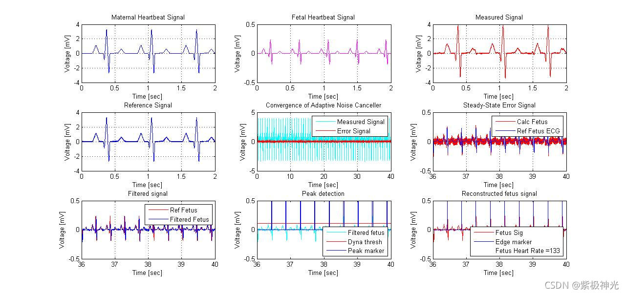
title(‘Reconstructed fetus signal’);
legend(‘Fetus Sig’,‘Edge marker’,fetus_bpm, ‘Location’,‘SouthEast’);
axis([Time-4 Time -0.5 0.5]);
## ⛄三、运行结果
## ⛄四、matlab版本及参考文献
**1 matlab版本**
2014a
**2 参考文献**
[1]焦运良,邢计元,靳尧凯.基于小波变换的心电信号阈值去噪算法研究[J].信息技术与网络安全. 2019,38(05)
**3 备注**
简介此部分摘自互联网,仅供参考,若侵权,联系删除