第1章 强化学习基础

1.1 强化学习基础（上）- Overview

What is reinforcement learning

a computational approach to learning whereby an agent tries to maximize the total amount of reward it receives while interacting with a complex and uncertain environment. -Sutton and Barto

Supervised Learning: Image Classification

• Annotated images, data follows i.i.d distribution.
• Learners are told what the labels are.

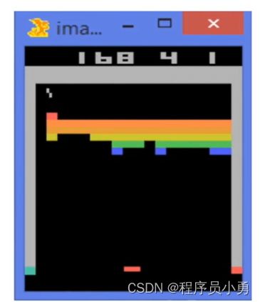
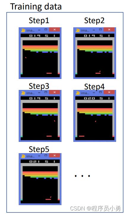
Reinforcement learning: Playing Breakout

• Data are not i,i,d. Instead, a correlated times series data
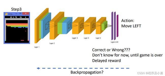
• No instant feedback or label for correct action

Action: Move LEFT or Right

Difference between Reinforcement learning and Supervised Learning

• Sequential data as input (not i.i.d)
• The learner is not told which actions to take, but instead must discover which actions yield the most reward by trying them.
• Trial-and-error exploration (balance between exploration and exploitation)
• There is no supervisor, only a reward signal, which is also delayed

Features of Reinforcement learning

• Trial-and-error exploration
• Delayed reward
• Time matters (sequential data, non i.i.d data)
• Agent’s actions affect the subsequent data it receives (agent’s action changes the environment)

Big deal: Able to Achieve Superhuman Performance

• Upper bound for Supervised Learning is human-performance.
• Upper bound for reinforcement learning?

https://www/youtube.com/watch?v=WXuK6gekU1Y

Examples of reinforcement learning

• A chess player makes a move: the choice is informed both by planning-anticipating possible replies and counterreplies.

  

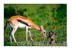
• A gazelle calf struggles to stand, 30 min later it runs 36 kilometers per hour.

  

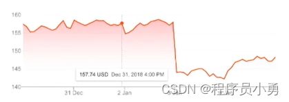
• Portfolio management.

  

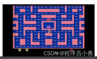
• Playing Atari game

  

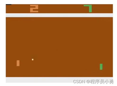
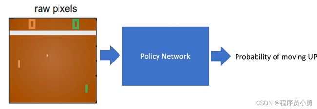
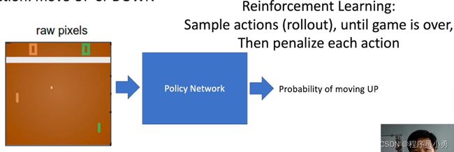
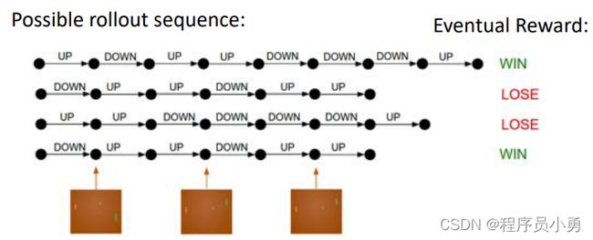
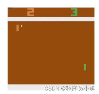
RL example: Pong

Action: move UP or Down

From Andrej Karpathy blog: http://karpathy.github.io/2016/05/31/rl/

Deep Reinforcement Learning: Deep Learning + Reinforcement Learning

• Analogy to traditional CV and deep CV

• Standard RL and deep RL

Why RL works now?

• Computation power: many GPUs to do rial-and-error exploration
• Acquire the degree of proficiency in domains governed by simple, known rules
• End-to-end training, features and policy are jointly optimized toward the end goal.

More Examples on RL

https://www.youtube.com/watch?v=gn4nRCC9TwQ

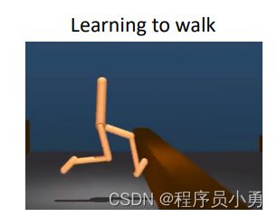
https://ai.googleblog.com/2016/03/deep-learning-for-robots-learning-from.html

https://www.youtube.com/watch?v=jwSbzNHGflM

https://www.youtube.com/watch?v=ixmE5nt2o88

1.2 强化学习基础（下）- Introduction to Sequential Decision Making

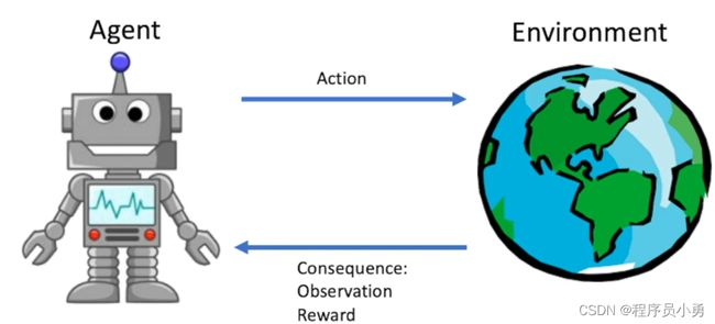
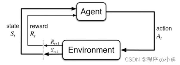
The agent learns to interact with the environment

Rewards

• A reward is a scalar feedback signal
• Indicate how well agent is doing at step t
• Reinforcement Learning is based on maximization of rewards:

All goals of agent can be described by the maximization of expected cumulative reward.

Examples of Rewards

• Chess player play to win:

+/- reward for winning or losing a game

• Gazelle calf struggles to stand:

+/- reward for running with its mom or being eaten

• Manage stock investment

+/- reward for each profit or loss in $

• Play Atari games

+/- reward for increasing or decreasing scores

Sequential Decision Making

• Objective of the agent: select a series of actions to maximize total future rewards

• Actions may have long term consequences

• Reward may be delayed

• Trade-off between immediate reward and long-term reward

• The history is sequence of observation, actions, rewards.
  $$H_t=O_1,R_1,A_1,...,A_{t-1},O_t,R_t$$

• What happens next depends on the history

• State is the function used to determine what happens next
  $$S_t=f(H_t)$$

• Environment state and agent state
  $$S_t^e=f^e(H_t)S_t^a=f^a(H_t)$$

• Full observability: agent directly observe the environment state, formally as Markov decision process (MDP)
  $$O_t=S_t^e=S_t^a$$

• Partial observability: agent indirectly observe the environment, formally as partial observable Markov decision process (POMDP)

  • Black jack (only see public cards), Atari game with pixel observation

Major Components of an RL Agent

An RL agent may include one or more of these components:

• Policy: agent’s behavior function
• Value function: how good is each state or action
• Model: agent’s state representation of the environment

Policy

• A policy is the agent’s behavior model
• It is a map function state/observation to action.
• Stochastic policy: Probabilistic sample $\pi (a|s)=P[A_t=a|S_t=s]$
• Deterministic policy: $a\ast =arg\underset{a}{\max }\pi (a|s)$

Value function

• Value function: expected discounted sum of future rewards under a particular policy $\pi$

• Discount factor weights immediate vs future rewards

• Used to quantify goodness/badness of states and actions
  $$v_{\pi }(s)\doteq E_{\pi }[G_t|S_t=s]=E_{\pi }[\sum _{k=0}^{\infty }{\gamma }^k{R}_{t+k+1}|S_t=s],foralls\in S$$

• Q-function (could be used to select among actions)
  $$q_{\pi }(s,a)\doteq E_{\pi }[G_t|S_t=s,A_t=a]=E_{\pi }[\sum _{k=0}^{\infty }{\gamma }^k{R}_{t+k+1}|S_t=s,A_t=a].$$

Model

A model predict what the environment will do next

predict the next state: $P_{S{S}^{\prime }}^a=\mathbb{P}[S_{t+1}=s^{\prime }|S_t=s],A_t=a$

Markov Decision Processes (MDPs)

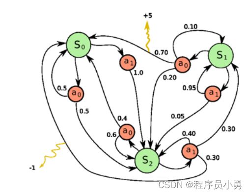
Definition of MDP

1. $P^a$ is dynamics/transition model for each action
   $$P(S_{t+1}=s^{\prime }|S_t=s,A_t=a)$$

2. R is reward function $R(S_t=s,A_t=a)=\mathbb{E}[R_t|S_t=s,A_t=a]$

3. Discount factor γ ∈ [0, 1]

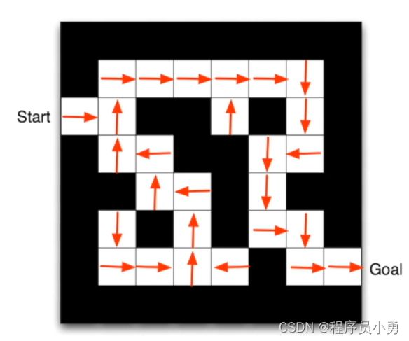
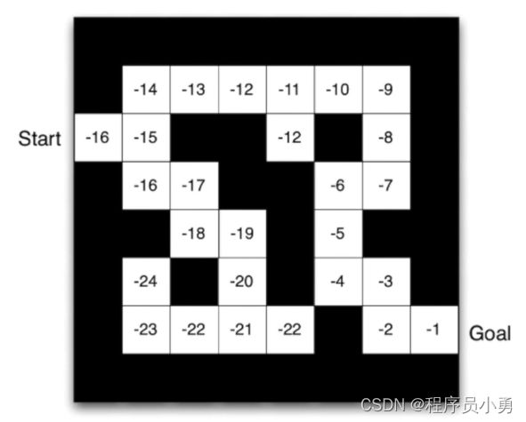
Maze Example

• Rewards: -1 per time-step
• Actions: N, E, S, W
• States: Agent’s location

From David Silver Slide

Maze Example: Result from Policy-based RL

• Arrows represent policy $\pi (s)$ for each state s

Maze Example: Result from Values-based RL

• Numbers represent value $v_{\pi (s)}$ for each state s

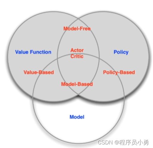
Types of RL Agents based on What the Agent Learns

• Values-based agent:
  • Explicit: Value function
  • Implicit: Policy (can derive a policy from value function)
• Policy-based agent:
  • Explicit: policy
  • No value function
• Actor-Critic agent:
  • Explicit: policy and value function

Types of RL Agents on if there is model

• Model-based
  • Explicit: model
  • May or may not have policy and/or value function
• Model-free
  • Explicit: value function and/or policy function
  • No model.

Types of RL Agents

Credit: David Silver’s slide

Exploration and Exploitation

• Agent only experiences what happens for the actions it tries!

• How should an RL agent balance its actions?

  • Exploration: trying new things that might enable the agent to make better decisions in the future
  • Exploitation: choosing actions that are expected to yield good reward given the past experience

• Often there may be an exploration-exploitation trade-off

  • May have to sacrifice reward in order to explore & learn about potentially better policy

• Restaurant Selection

  • Exploitation: Go to your favourite restaurant
  • Exploration: Try a new restaurant

• Online Banner Advertisements

  • Exploitation: Show the most successful advert
  • Exploration: Show a different advert

• Oil Drilling

  • Exploitation: Drill at the best-known location
  • Exploration: Drill at a new location

• Game Playing

  • Exploitation: Play the move you believe is
  • Exploration: play an experimental move

Coding

https://github.com/metalbubble/RLexample

OpenAI: specialized in Reinforcement Learning

• https://openai.com/
• OpenAI is a non-profit AI research company, discovering and enacting the path to safe artificial general intelligence (AGI).

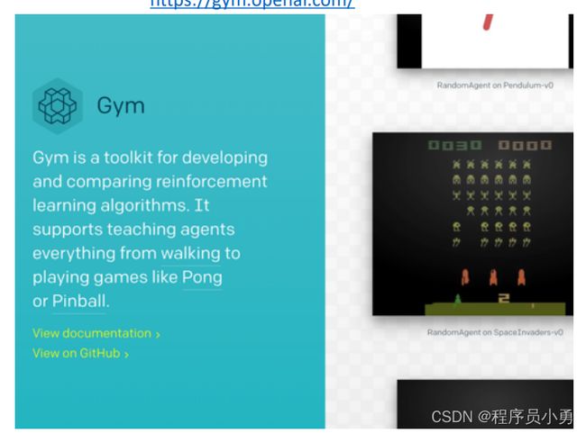
OpenAI gym library

https://github.com/openai/retro

Algorithmic interface of reinforcement learning

import gym
env = gym.make("Taxi-v2")
observation = env.reset()
agent = load_agent()
for step in range(100):
    action = agent(observation)
    observation, reward, done, info = env.step(action) 

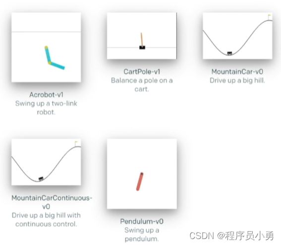
Classic Control Problems

https://gym.openai.com/envs/#classic_control

Example of CartPole_v0

https://github.com/openai/gym/blob/master/gym/envs/classic_control/cartpole.py

Example code

import gym
env = gym.make("CartPole-v0")
env.reset()
env.render() # display the rendered scene
action = env.action_space.sample()
observation, reward, done, info = env.step(action)  

Cross Entropy method(CEM)

https://gist.github.com/kashif/5dfa12d80402c559e060d567ea352c06

Deep Reinforcement Learning Example

• Pong example

import gym
env = gym.make("Pong-v0")
env.reset()
env.render() # display the rendered scene

python my_random_agent.py Pong-v0

python pg-pong.py

Loading weight: pong_bolei.p(model trained over night)

• Look deeper into the code

observation = env.reset()

cur_x = prepro(observation)
x = cur_x - pre_x
pre_x = cur_x
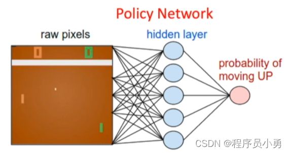
aprob, h = policy_forward(x)

Randomized action:
    action = 2 if np.random.uniform() < aprob else 3 # roll the dice!

h = np.dot(W1, x)
h[h<0] = 0 # ReLU nonlinearity: threshold at zero
logp = np.dot(W2,h) # compute log probability of going up
p = 1.0 / (1.0 + np.exp(-logp)) #sigmoid function (gives probability of going up)

How to optimize the W1 and W2?

Policy Gradient！（To be introduced in future lecture）

http://karpathy.github.io/2016/05/31/rl

Homework and What’s Next

• Play with OpenAI gym and the example code

https://github.com/cuhkrlcourse/RLexample

• Go through this blog in detail to understand pg-pong.py

http://karpathy.github.io/2016/05/31/rl

• Next week: Markov Decision Process

Please read Sutton and Barton: Chapter 1 and Chapter 3