最大似然法监督分类步骤_数据科学：AdaBoost分类器

> image:BBVA

介绍：

Boosting是一种集成技术，用于从多个弱分类器创建强分类器。 集成技术的一个众所周知的例子是随机森林(Random Forest)，它使用多个决策树来创建一个随机森林。

直觉：

AdaBoost，Adaptive Boosting的缩写，是第一个成功的针对二进制分类开发的Boosting算法。它是一种监督式机器学习算法，用于提高任何机器学习算法的性能。 最好与像决策树这样的弱学习者一起使用。 这些模型在分类问题上的准确性要高于随机机会。

AdaBoost的概念很简单：

我们将把数据集传递给多个基础学习者，每个基础学习者将尝试更正其前辈分类错误的记录。

我们会将数据集(如下所示，所有行)传递给Base Learner1。所有被Base Learner 1误分类的记录(行5,6和7被错误分类)将被传递给Base Learner 2，类似地，所有Base分类器的错误分类记录 学习者2将被传递给基本学习者3。最后，根据每个基本学习者的多数票，我们将对新记录进行分类。

让我们逐步了解AdaBoost分类器的实现：

步骤1：获取数据集，并将初始权重分配给指定数据集中的所有样本(行)。

W = 1 / n => 1/7，其中n是样本数。

步骤2：我们将创建第一个基础学习器。在AdaBoost中，我们将决策树用作基础学习器。这里要注意的是，我们将仅创建深度为1的决策树，它们被称为决策树桩或树桩。

我们将为数据集的每个特征创建一个树桩，就像在我们的例子中，我们将创建三个树桩，每个特征一个。

步骤3：我们需要根据每个特征的熵值或吉尼系数，选择任何基础学习器模型(为特征1创建的基础学习器1，为特征2创建的基础学习器2，为特征3创建的基础学习器3) (我在决策树文章中已经讨论了Ginni和熵)。

熵或吉尼系数值最小的基础学习器，我们将为第一个基础学习器模型选择该模型。

第4步：我们需要找到在第3步中选择的基本学习者模型正确分类了多少条记录以及错误分类了多少条记录。

我们必须找到所有错误分类的总错误，让我们说我们是否正确分类了4条记录而错误分类了1条记录

Total Error =分类错误的记录的样本权重的总和。

因为我们只有1个错误，所以总错误= 1/7

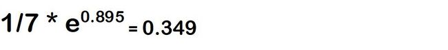
步骤5：通过以下公式检查树桩的性能。

当我们将Total Error放入该公式时，我们将得到0.895的值(不要偷懒地将这些值进行计算)

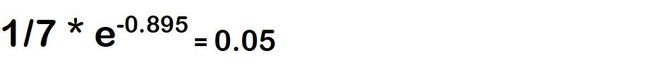
通过以下等式更新正确和错误分类的样本(行)的样本权重。

错误分类的样本的新样本权重=

正确分类的样本的新样本权重=

注意：我们假设第3行的分类不正确

步骤6：我们在这里考虑的要点是，当我们将所有样本权重相加时，它等于1，但如果更新了权重，则总和不等于1。因此，我们将每个更新的权重除以总和，然后归一化 值为1。

更新权重的总和是0.68

第7步：我们将通过删除"样品重量"和"更新重量"功能来创建数据集，并将每个样品(行)分配到一个桶中。

步骤8：建立新的资料集。 为此，我们必须从0到1(对于每个样本(行))中随机选择一个值，然后选择该样本，该样本在" Bucket"下掉落，并将该样本保留在" NEW DATASET"中。 由于分类错误的记录具有较大的存储桶大小，因此选择该记录的可能性非常高。

我们在这里可以看到，由于数据桶大小比其他行大，因此已在我们的数据集中选择了3次错误分类的record(Row3)。

第9步：为下一个树桩(基础学习者2，基础学习者3)获取此新数据集，并按照步骤1至8进行所有功能。

Adaboost模型通过让森林中的每棵树对样本进行分类来进行预测。然后，根据树木的决策将它们分成几组。现在，对于每组，我们对各树中每棵树的重要性进行累加。 整个森林的数量由总和最大的群体决定。下图。

Adaboost分类器的逐步Python代码：

In [1]:#General idea behind boosting methods is to train predictors sequentially,each trying to correct its predecessor# AdaBoost Classifier Example In Python# Step 1: Initialize the sample weights# Step 2: Build a decision tree with each feature, classify the data and evaluate the result# Step 3: Calculate the significance of the tree in the final classification# Step 4: Update the sample weights so that the next decision tree will take the errors made by the preceding decision tree into account# Step 5: Form a new dataset# Step 6: Repeat steps 2 through 5 until the number of iterations equals the number specified by the hyperparameter (i.e. number of estimators)# Step 7: Use the forest of decision trees to make predictions on data outside of the training setIn [2]:from sklearn.ensemble import AdaBoostClassifierfrom sklearn.tree import DecisionTreeClassifierfrom sklearn.datasets import load_breast_cancerimport pandas as pdimport numpy as npimport seaborn as snsimport matplotlib.pyplot as pltfrom sklearn.model_selection import train_test_splitfrom sklearn.metrics import confusion_matrix,accuracy_scorefrom sklearn.preprocessing import LabelEncoderimport warningswarnings.filterwarnings('ignore')In [3]:cancer_data=load_breast_cancer()In [4]:X=pd.DataFrame(cancer_data.data,columns=cancer_data.feature_names)In [5]:y = pd.Categorical.from_codes(cancer_data.target, cancer_data.target_names)In [6]:#y=pd.DataFrame(y,columns=['Cancer_Target'])Data PreprocessingIn [7]:X.describe()Out[7]:mean radiusmean texturemean perimetermean areamean smoothnessmean compactnessmean concavitymean concave pointsmean symmetrymean fractal dimension...worst radiusworst textureworst perimeterworst areaworst smoothnessworst compactnessworst concavityworst concave pointsworst symmetryworst fractal dimensioncount569.000000569.000000569.000000569.000000569.000000569.000000569.000000569.000000569.000000569.000000...569.000000569.000000569.000000569.000000569.000000569.000000569.000000569.000000569.000000569.000000mean14.12729219.28964991.969033654.8891040.0963600.1043410.0887990.0489190.1811620.062798...16.26919025.677223107.261213880.5831280.1323690.2542650.2721880.1146060.2900760.083946std3.5240494.30103624.298981351.9141290.0140640.0528130.0797200.0388030.0274140.007060...4.8332426.14625833.602542569.3569930.0228320.1573360.2086240.0657320.0618670.018061min6.9810009.71000043.790000143.5000000.0526300.0193800.0000000.0000000.1060000.049960...7.93000012.02000050.410000185.2000000.0711700.0272900.0000000.0000000.1565000.05504025%11.70000016.17000075.170000420.3000000.0863700.0649200.0295600.0203100.1619000.057700...13.01000021.08000084.110000515.3000000.1166000.1472000.1145000.0649300.2504000.07146050%13.37000018.84000086.240000551.1000000.0958700.0926300.0615400.0335000.1792000.061540...14.97000025.41000097.660000686.5000000.1313000.2119000.2267000.0999300.2822000.08004075%15.78000021.800000104.100000782.7000000.1053000.1304000.1307000.0740000.1957000.066120...18.79000029.720000125.4000001084.0000000.1460000.3391000.3829000.1614000.3179000.092080max28.11000039.280000188.5000002501.0000000.1634000.3454000.4268000.2012000.3040000.097440...36.04000049.540000251.2000004254.0000000.2226001.0580001.2520000.2910000.6638000.2075008 rows × 30 columnsIn [8]:X.isnull().count()Out[8]:mean radius                569mean texture               569mean perimeter             569mean area                  569mean smoothness            569mean compactness           569mean concavity             569mean concave points        569mean symmetry              569mean fractal dimension     569radius error               569texture error              569perimeter error            569area error                 569smoothness error           569compactness error          569concavity error            569concave points error       569symmetry error             569fractal dimension error    569worst radius               569worst texture              569worst perimeter            569worst area                 569worst smoothness           569worst compactness          569worst concavity            569worst concave points       569worst symmetry             569worst fractal dimension    569dtype: int64In [9]:def heatMap(df):    #Create Correlation df    corr = X.corr()    #Plot figsize    fig, ax = plt.subplots(figsize=(25, 25))    #Generate Color Map    colormap = sns.diverging_palette(220, 10, as_cmap=True)    #Generate Heat Map, allow annotations and place floats in map    sns.heatmap(corr, cmap=colormap, annot=True, fmt=".2f")    #Apply xticks    plt.xticks(range(len(corr.columns)), corr.columns);    #Apply yticks    plt.yticks(range(len(corr.columns)), corr.columns)    #show plot    plt.show()In [10]:heatMap(X)All the above correlated features can be droppedIn [11]:X.boxplot(figsize=(10,15))Out[11]:In [12]:le=LabelEncoder()In [13]:y=pd.Series(le.fit_transform(y))Data Split and Model InitializationIn [14]:X_train,X_test,y_train,y_test=train_test_split(X,y,test_size=0.20,random_state=42)In [15]:adaboost=AdaBoostClassifier(DecisionTreeClassifier(max_depth=1),n_estimators=200)In [16]:adaboost.fit(X_train,y_train)Out[16]:AdaBoostClassifier(algorithm='SAMME.R',          base_estimator=DecisionTreeClassifier(class_weight=None, criterion='gini', max_depth=1,            max_features=None, max_leaf_nodes=None,            min_impurity_decrease=0.0, min_impurity_split=None,            min_samples_leaf=1, min_samples_split=2,            min_weight_fraction_leaf=0.0, presort=False, random_state=None,            splitter='best'),          learning_rate=1.0, n_estimators=200, random_state=None)In [17]:adaboost.score(X_train,y_train)Out[17]:1.0In [18]:adaboost.score(X_test,y_test)Out[18]:0.9736842105263158In [19]:y_pred=adaboost.predict(X_test)In [20]:y_predOut[20]:array([0, 1, 1, 0, 0, 1, 1, 1, 1, 0, 0, 1, 0, 1, 0, 1, 0, 0, 0, 1, 0, 0,       1, 0, 0, 0, 0, 0, 0, 1, 0, 0, 0, 0, 0, 0, 1, 0, 1, 0, 0, 1, 0, 0,       0, 0, 0, 0, 0, 0, 1, 1, 0, 0, 0, 0, 0, 1, 1, 0, 0, 1, 1, 0, 0, 0,       1, 1, 0, 0, 1, 1, 0, 1, 0, 0, 0, 0, 0, 0, 1, 0, 1, 1, 1, 1, 1, 1,       0, 0, 0, 0, 0, 0, 0, 0, 1, 1, 0, 1, 1, 0, 1, 1, 0, 0, 0, 1, 0, 0,       1, 0, 0, 1])Result VisualizationIn [21]:cm=confusion_matrix(y_test,y_pred)print('Confusion Matrix {} '.format(cm))Confusion Matrix [[70  1] [ 2 41]] In [22]:ax= plt.subplot()sns.heatmap(cm, annot=True, ax = ax);# labels, title and ticksax.set_xlabel('Predicted labels');ax.set_ylabel('True labels'); ax.set_title('Confusion Matrix');In [23]:acc=accuracy_score(y_test,y_pred)print('Model Accuracy is {} % '.format(round(acc,3)))Model Accuracy is 0.974 % 

AdaBoost分类器的优点：

· AdaBoost可用于提高弱分类器的准确性，从而使其更灵活。 现在，它已扩展到二进制分类之外，并且还发现了文本和图像分类中的用例。

· AdaBoost具有很高的精度。

· 不同的分类算法可以用作弱分类器。

缺点：

· 提升技巧是逐步学习的，确保您拥有高质量的数据非常重要。

· AdaBoost对噪声数据和异常值也非常敏感，因此，如果您打算使用AdaBoost，则强烈建议消除它们。

· AdaBoost还被证明比XGBoost慢。

结论：在本文中，我们讨论了理解AdaBoost算法的各种方法.AdaBoost就像是一个恩赐，如果正确使用它可以提高分类算法的准确性。

希望您喜欢我的文章。请鼓掌(最多50次)，这会激发我写更多的文章。

(本文翻译自Anjani Kumar的文章《Data Science : AdaBoost Classifier》，参考：https://medium.com/datadriveninvestor/data-science-adaboost-classifier-4879a45c4300)