Machine Learning with Graphs 之 Message Passing and Node Classification

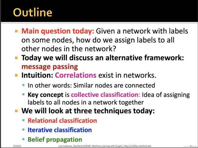
In network theory, collective classification is the simultaneous prediction of the labels for multiple objects, where each label is predicted using information about the object’s observed features, the observed features and labels of its neighbors, and the unobserved labels of its neighbors.[1] Collective classification problems are defined in terms of networks of random variables, where the network structure determines the relationship between the random variables. Inference is performed on multiple random variables simultaneously, typically by propagating information between nodes in the network to perform approximate inference. Approaches that use collective classification can make use of relational information when performing inference. Examples of collective classification include predicting attributes (ex. gender, age, political affiliation) of individuals in a social network, classifying webpages in the World Wide Web, and inferring the research area of a paper in a scientific publication dataset.
https://en.wikipedia.org/wiki/Collective_classification

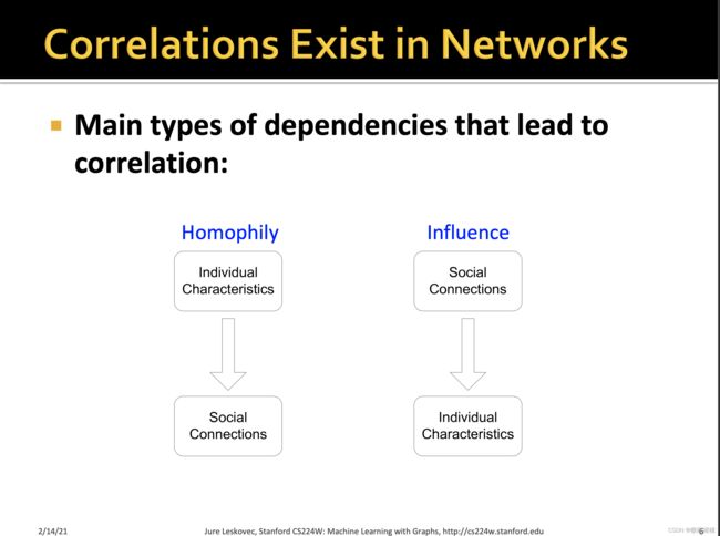
Homophily is the principle that a contact between similar people occurs at a higher rate than among dissimilar people. The pervasive fact of homophily means that cultural, behavioral, genetic, or material information that flows through net- works will tend to be localized.

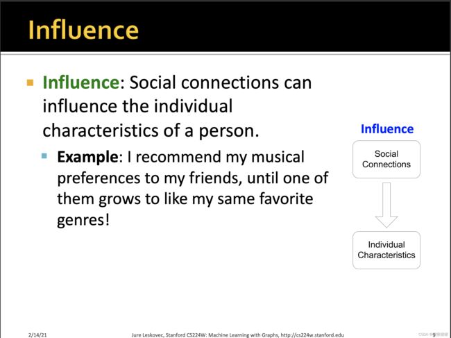
前者可以理解为物以类聚，人以群分
后者可以理解为橘生淮南则为橘生于淮北则为枳 || 近朱者赤近墨者黑
两者是可以相互影响循环的

guilt-by-association可以翻译为连坐 or 关联推断

A very disconcerting practice is documented by various sources - collective punishment based upon “guilt by association”.各种资料来源记录了一种很令人不安的做法，即以" 连坐罪" 为依据的集体处罚。

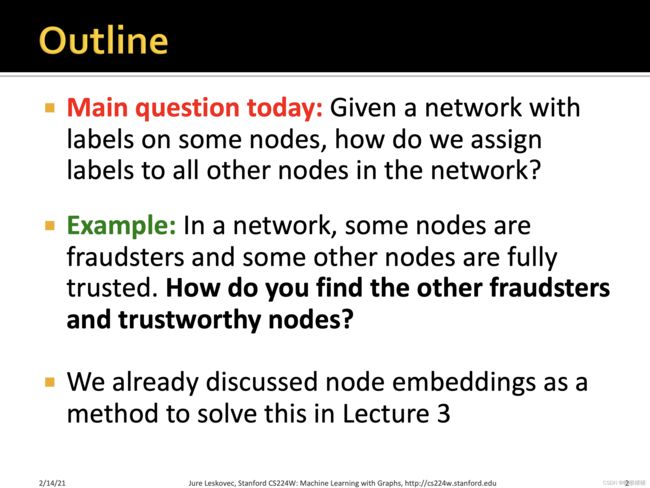
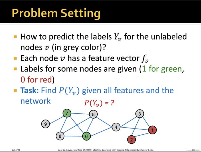
因此，如何根据已知的节点，对未知的节点进行标签分类呢？
这儿，主要有两个出发点
【1】相似的节点往往很接近或者直接相连
【2】对于一个节点进行标签分类，往往取决于节点本身的特征，以及其邻居节点的特征以及标签。
也可以进行多标签分类，比如对一个人的多个属性进行预测，当然可以将多分类转化为多个二分类。

马尔可夫假设，即节点的标签只取决于它的邻接节点的标签

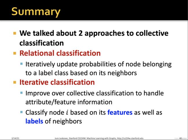
Collective classification 分为如下三步进行：
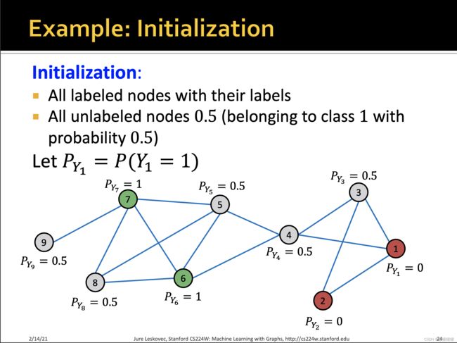
【1】Local classifier : 标签初始化，仅仅依赖于节点自身的信息
【2】relational classifier：利用了邻居节点的标签和特征
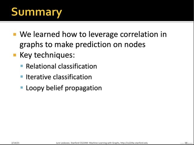
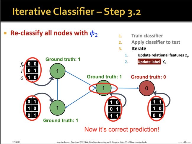
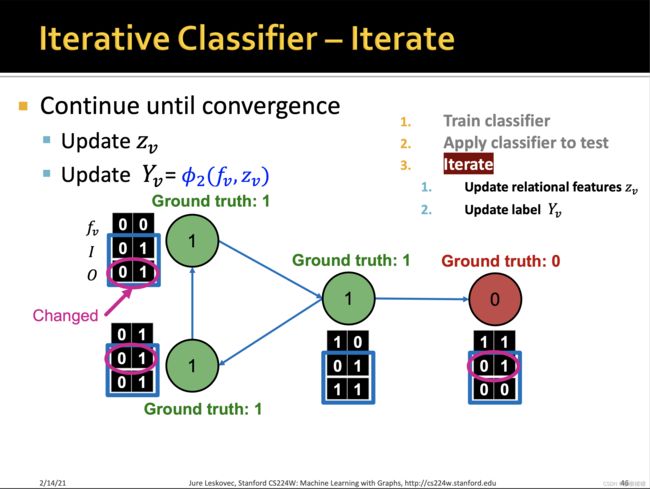
【3】collective inference：迭代地将correlation进行传播（应用classifier到每个节点身上），直到收敛或者达到最大次数

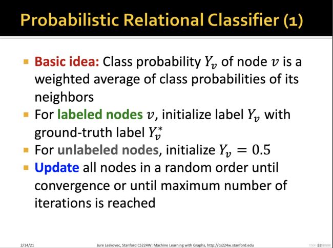
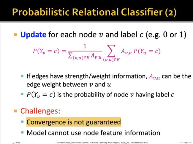
import numpy as np
def prc(x, A, max_iters = 100):
    '''
    This function will perform the probabilistic relational algorithm on a given vector x and the associated
    adjacent matrix of the network

    args:
        x (Array) : Initial vector
        A (Matrix) : Input adjacent matrix
        max_iters (Integer) : The maximum number of iterations

    returns:
        This function will return the result vector x
    '''
    err = 1.0
    old_x = x
    for i in range(max_iters):
        x = A.dot(x)
        d = A.sum(axis = 1)
        x = np.divide(x,d)
        x = np.around(x,2)
        x[0] = 0
        x[1] = 0
        x[5] = 1
        x[6] = 1
        err = np.linalg.norm(x - old_x, 1)
        if err <= 1e-6:
            break
        old_x = x
        print(list(x))
    return x

if __name__ == "__main__":
    A = [[0,1,1,1,0,0,0,0,0],
         [1,0,1,0,0,0,0,0,0],
         [1,1,0,1,0,0,0,0,0],
         [1,0,1,0,1,1,0,0,0],
         [0,0,0,1,0,1,1,1,0],
         [0,0,0,1,1,0,1,1,0],
         [0,0,0,0,1,1,0,1,1],
         [0,0,0,0,1,1,1,0,0],
         [0,0,0,0,0,0,1,0,0]]
    x = [0,0,0.5,0.5,0.5,1,1,0.5,0.5]
    A = np.array(A)
    x = np.array(x)
    x = prc(x, A, 20)

[0.0, 0.0, 0.17, 0.5, 0.75, 1.0, 1.0, 0.83, 1.0]
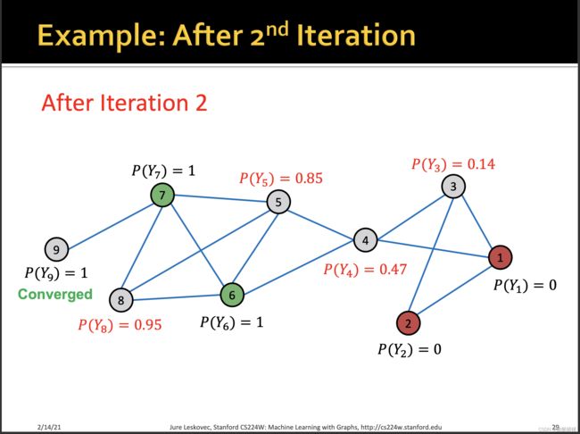
[0.0, 0.0, 0.17, 0.48, 0.83, 1.0, 1.0, 0.92, 1.0]
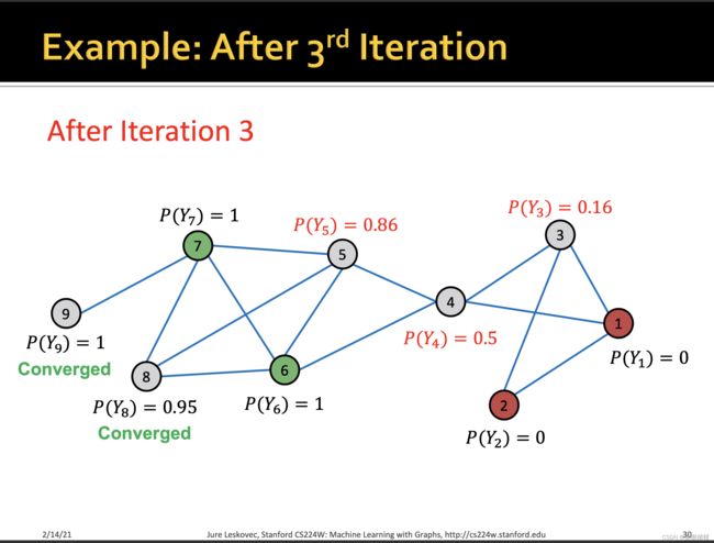
[0.0, 0.0, 0.16, 0.5, 0.85, 1.0, 1.0, 0.94, 1.0]
[0.0, 0.0, 0.17, 0.5, 0.86, 1.0, 1.0, 0.95, 1.0]
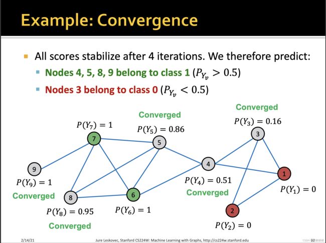
[0.0, 0.0, 0.17, 0.51, 0.86, 1.0, 1.0, 0.95, 1.0]

P(Y3)有一点差异不知道为什么

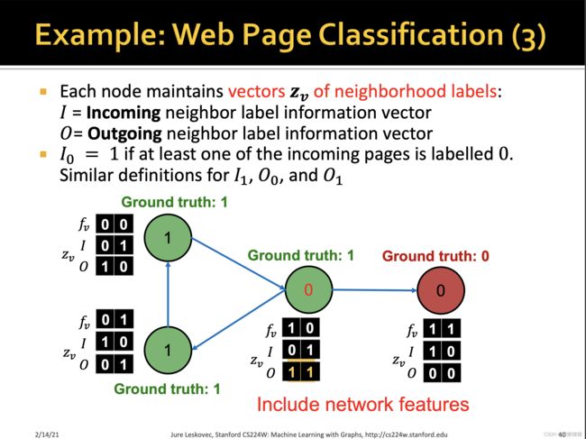
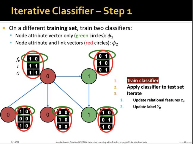
训练两个分类器：
【1】第一个分类器器基于节点本身的特征，预测节点的标签
【2】第二个分类器基于节点的特征和邻居标签的summary来预测节点的标签。
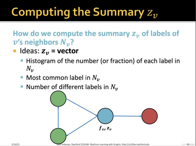summary有多种计算方式






置信传播
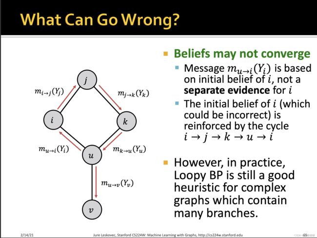
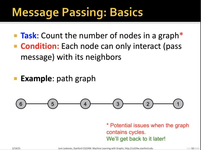
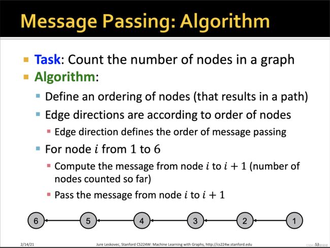
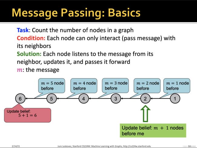
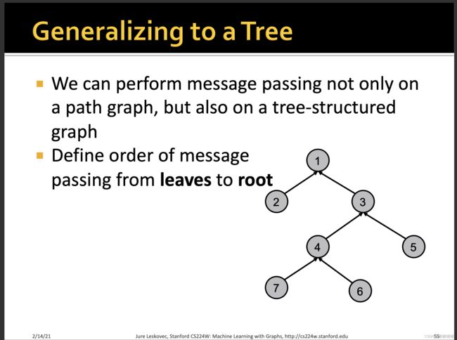
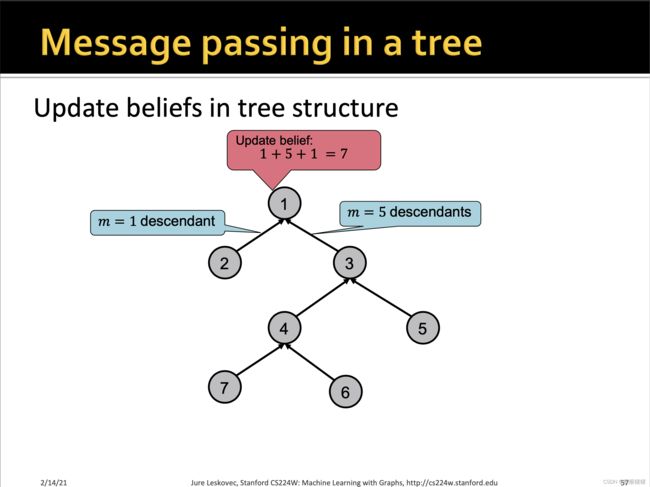
Belief Propagation 算法（BP算法）是将概率论应用到图结构中的一种动态规划的算法。在迭代过程中，相邻的节点相互交换“信息”（passing message）。当相邻节点“达成共识（When consensus is reached）”，计算最后的置信值（belief）。
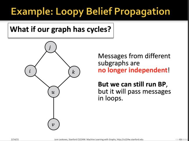
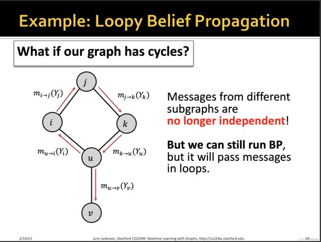
Loopy Belief Propagation环路置信传播





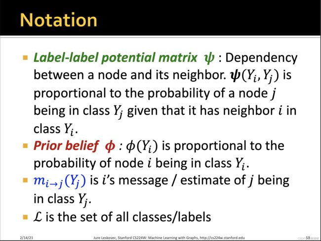$\varphi (Y_i,Y_j)=\alpha .P(Y_j|Y_i)$，节点与它邻居节点的相关性正比于如下的条件概率，即已知i的标签为$Y_i$的情况下，j的标签是$Y_j$的概率。
比如对于一个二分类而言
它的potential matrix如果是如下的情况

0.2	0.8
0.4	0.6

就意味着，如果i的标签是0，那么j的标签是1的概率是0.8.
如果i的标签是1，那么j的标签是1的概率是0.6 ？
这意味着如果对角线上的值越大，j如果属于标签1，那么i的标签也更有可能属于标签1，反之，如果对角线上的值越小，那么两者的标签相反的可能性更大
如果i的先验概率 $\varphi (Y_i)$为 $\varphi (0)$ = 0.3 $\varphi (1)$ = 0.7
那么i’s message/estimate of j being in class $Y_j=0$的计算方式如下
p0 = All meassage sent by i’s neighbors from previous round that belive i belongs to 0
p1 = All meassage sent by i’s neighbors from previous round that belive i belongs to 1
下面忽略 $\alpha$
$m_{i2j}(Y_j=0)=0.2\ast 0.3\ast p0+0.4\ast 0.7\ast p1$
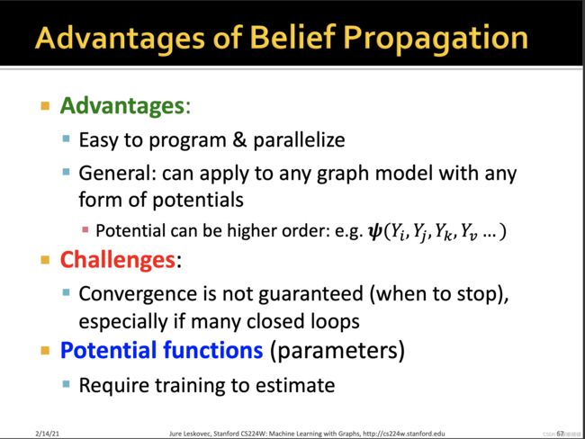
而上面这种potential matrix，往往是需要用数据训练来估计得到的
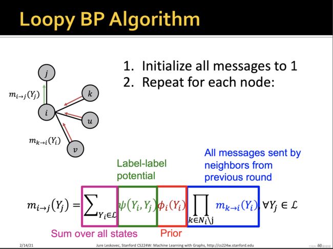all message sent by neighbors from previois roud, namely sum over every but j.