论文笔记：Enhanced LSTM for Natural Language Inference

Enhanced LSTM for Natural Language Inference

https://arxiv.org/pdf/1609.06038v3.pdf

Related Work

• Enhancing sequential inference models based on chain networks
• Further, considering recursive architectures to encode syntactic parsing information

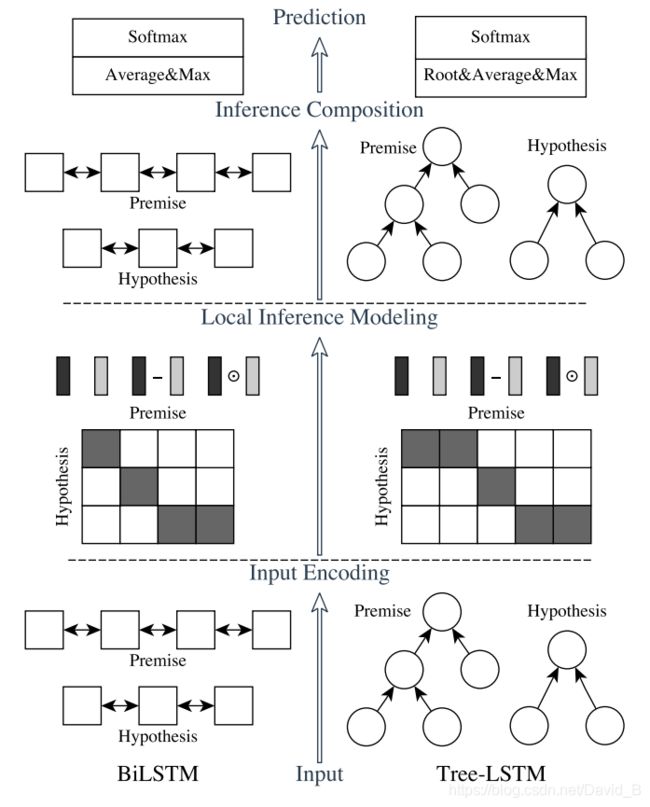
Hybrid Neural Inference Models

Major components

• input encoding、local inference modeling、inference composition
• ESIM（sequential NLI model）、Tree LSTM（incorporate syntactic parsing information）
  

Notation

• Two sentences:
  • $a=(a_1,...,a_{l_a})$
  • $b=(b_1,...,b_{l_b})$
• Enbedding of $l$-dimensional vector: $a_i$、$b_j\in {\mathbb{R}}^l$
• ${\bar{a}}_i$: generated by the $BiLSTM$ at time $i$ over the input sequence $a$

Goal

• Predict a label $y$ that indicates the logic relationship between $a$ and $b$

Input Encoding

• Use $BiLSTM$ to encode the input premise and hypothesis

• Hidden states by two LSTMs at each time step are concatenated to represent that time step and its context

• Encode syntactic parse trees of a premise and hypothesis through tree-LSTM

• A tree node is deployed with a tree-LSTM memory block depicted

  • At each node, an input vector $x_t$ and hidden vectors of it（$h_{t-1}^L$ and $h_{t-1}^R$）are taken in as the input to calculate the current node’s hidden vector $h_t$
    

• Detailed computation:

  • $h_t=TrLSTM(x_t,h_{t-1}^L,h_{t-1}^R)$
  • $h_t=o_t\odot tanh(c_t)$
  • $o_t=\sigma (W_o{x}_t+U_o^L{h}_{t-1}^L+U_o^R{h}_{t-1}^R)$
  • $c_t=f_t^T\odot c_{t-1}^L+f_t^R\odot c_{t-1}^R+i_t\odot u_t$
  • $f_t^L=\sigma (W_f{x}_t+U_f^{LL}{h}_{t-1}^L+U_f^{LR}{h}_{t-1}^R)$
  • $f_t^R=\sigma (W_f{x}_t+U_f^{RL}{h}_{t-1}^L+U_f^{RR}{h}_{t-1}^R)$
  • $i_t=\sigma (W_i{x}_t+U_i^L{h}_{t-1}^L+U_i^R{h}_{t-1}^R)$
  • $u_t=tanh(W_c{x}_t+U_c^L{h}_{t-1}^L+U_c^R{h}_{t-1}^R)$

• All $W\in {\mathbb{R}}^{d\times l},U\in d\times d$ are weight matrices to be learned

Local Inference Modeling

Locality of inference

• Employ some forms of hard or soft alignment to associate the relevant subcomponents between a premise and a hypothesis
• Argue for leveraging attention over the bidirectional sequential encoding of the input
• soft alignment layer computes the attention weights as the similarity of a hidden state tuple$<{\bar{a}}_i,{\bar{b}}_j>$ between a premise and a hypothesis with $e_{ij}={\bar{a}}_i^T{\bar{b}}_j$
• use bidirectional LSTM and tree-LSTM to encode the premise and hypothesis
• In sequential inference model, use BiLSTM

Local inference collected over sequences

• Local inference is determined by the attentiion weight $e_{ij}$, which is used to obtain the local relevance between a premise and hypothesis
• The content in ${\{{\bar{b}}_j\}}_{j=1}^{l_b}$ that is relevant to ${\bar{a}}_i$ will be selected and represented as ${\tilde{a}}_i$

${\tilde{a}}_i=\sum _{j=1}^{l_b}\frac{exp(e_{ij})}{{\sum }_{k=1}^{l_b}exp(e_{ik})}{\bar{b}}_j,\forall i\in [1,...,l_a]$

${\tilde{b}}_j=\sum _{i=1}^{l_a}\frac{exp(e_{ij})}{{\sum }_{k=1}^{l_a}exp(e_{kj})}{\bar{a}}_i,\forall j\in [1,...,l_b]$

Local inference collected over parse trees

• compute the difference and the element-wise product for the tuple $<\bar{a},\tilde{a}>$as well as for
  $<\bar{b},\tilde{b}>$
• The difference and element-wise product are then concatenated with the original vectors

$m_a=[\bar{a};\tilde{a};\bar{a}-\tilde{a};\bar{a}\odot \tilde{a};]$

$m_b=[\bar{b};\tilde{b};\bar{b}-\tilde{b};\bar{b}\odot \tilde{b};]$

Inference Composition

• Explore a composition layer to compose the enhanced local inference information $m_a$ and $m_b$

The composition layer

• In sequential inference model, use BiLSTM to compose local inference information sequentially
• Formulas for BiLSTM are used to capture local inference information $m_a$ and $m_b$ and their context here for inference composition
• In the tree composition, a tree node updates to compose local inference

$v_{a,t}=TrLSTM(F(m_{a,t}),h_{t-1}^L,h_{t-1}^R)$

$v_{b,t}=TrLSTM(F(m_{b,t}),h_{t-1}^L,h_{t-1}^R)$

• Use a 1-layer feedforward neural network with the ReLU activation, which is also applied to BiLSTM in sequential inference composition

Pooling

• Convert the resulting vectors obtained above to a fixed-length vector with pooling and feeds it to the final classifier to determine the overall inference relationship
• Compute both average and max pooling, and concatenate all these vectors to form the final fixed length vector $v$

$v_{a,ave}=\sum _{i=1}^{l_a}\frac{v_{a,i}}{l_a}$, $v_{a,max}=\underset{i=1}{\overset{l_a}{\max }}{v}_{a,i}$

$v_{b,ave}=\sum _{j=1}^{l_b}\frac{v_{b,j}}{l_b}$, $v_{b,max}=\underset{j=1}{\overset{l_b}{\max }}{v}_{b,j}$

$v=[v_{a,ave};v_{a,max};v_{b,ave};v_{b,max}]$

• Put $v$ into a final multilayer perceptron(MLP) classifier
• Use multi-class cross-entropy loss