逻辑回归（对数几率回归）推导及python代码实现

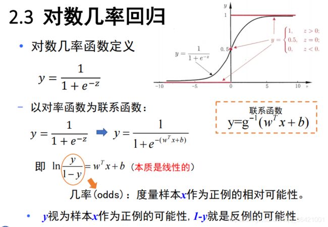
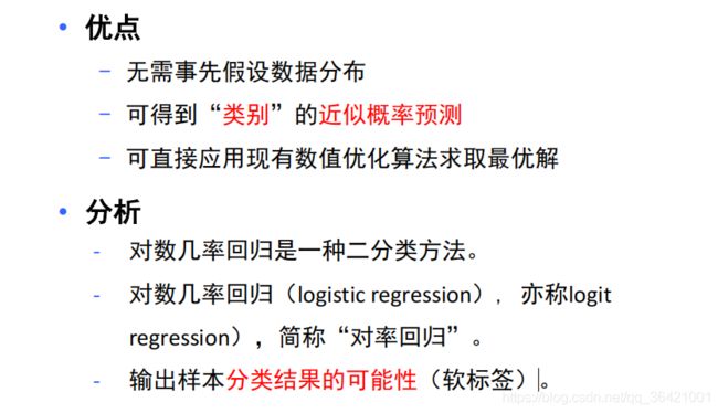
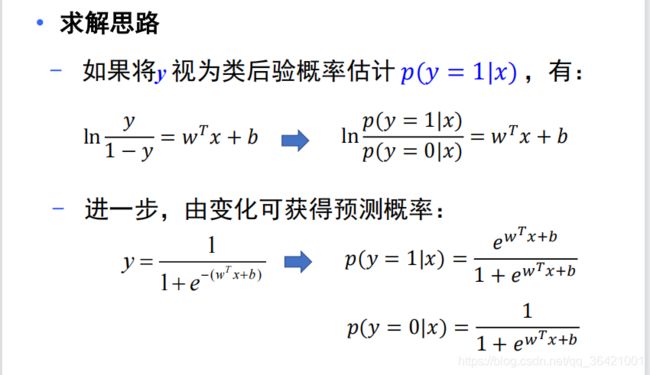
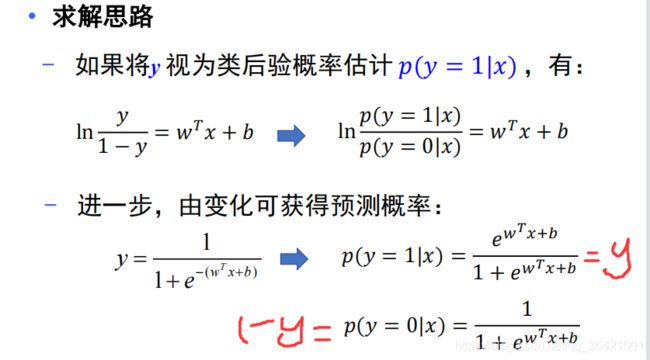
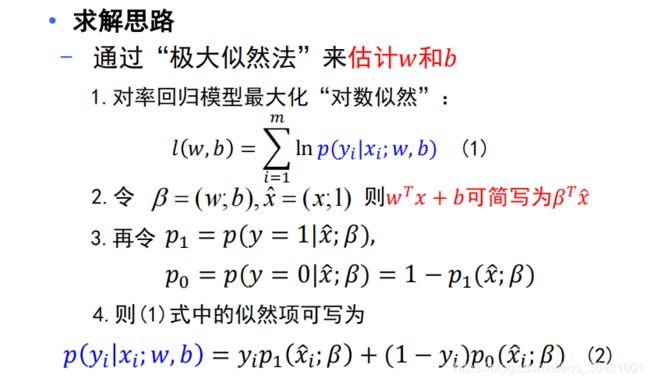
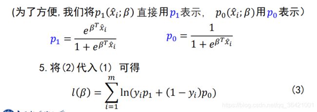
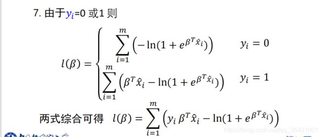
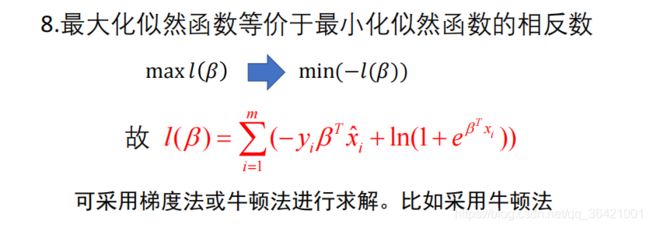
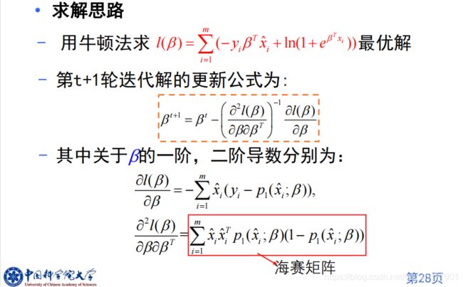
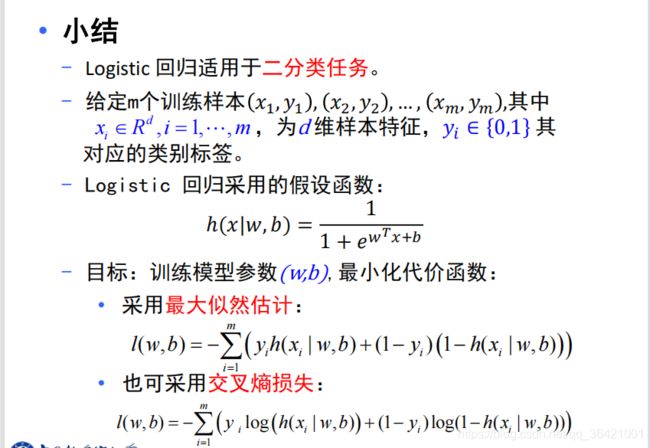
逻辑回归，也叫对数几率回归：

import numpy as np
import matplotlib.pyplot as plt
from sklearn.datasets._samples_generator import make_classification

class logistic_regression():
    def __init__(self):
        pass

    # 先定义一个sigmoid函数
    def sigmoid(self,x):
        z = 1 / (1 + np.exp(-x))
        return z

    # 定义模型参数初始化函数
    def initialize_param(self,dims):
        w = np.zeros((dims, 1))
        b = 0
        return w, b

    # 定义逻辑回归模型主体部分，包括模型计算公式，损失函数和参数的梯度公式
    def logistic(self,x, y, w, b):
        num_train = x.shape[0]
        num_feature = x.shape[1]

        a = self.sigmoid(np.dot(x, w) + b)#预测值
        #损失函数
        cost = -1 / num_train * np.sum(y * np.log(a) + (1 - y) * np.log(1 - a))
        #可基于上式分别关于 W 和b 求其偏导可得：
        dw = np.dot(x.T, (a - y)) / num_train
        db = np.sum(a - y) / num_train
        cost = np.squeeze(cost)
        return a, cost, dw, db

    #定义基于梯度下降的参数更新训练过程
    def logistic_train(self,x, y, learning_rate, epochs):
        # 初始化模型参数
        w, b = self.initialize_param(x.shape[1])
        cost_list = []
        # 迭代训练
        for i in range(epochs):
            # 计算当前迭代模型的计算结果，损失和参数梯度
            a, cost, dw, db = self.logistic(x, y, w, b)
            # 参数更新
            w = w - learning_rate * dw
            b = b - learning_rate * db
            # 记录损失，打印训练过程中的损失
            if i % 100 == 0:
                cost_list.append(cost)
                print('epoch %d cost %f' % (i, cost))
        # 保存参数
        params = {
            'w': w,
            'b': b
        }
        # 保存梯度
        grads = {
            'dw': dw,
            'db': db
        }
        return cost_list, params, grads

    def predict(self,x, params):
        y_prediction = self.sigmoid(np.dot(x, params['w']) + params['b'])
        for i in range(len(y_prediction)):
            if y_prediction[i] > 0.5:#预测结果大于0.5，则分为1类
                y_prediction[i] = 1
            else:
                y_prediction[i] = 0#预测结果小于0.5，则分为0类
        return y_prediction
        
#    定义一个分类准确率函数对训练集和测试集的准确率进行评估：
    def accuracy(self,y_test, y_pred):
        correct_count = 0
        for i in range(len(y_test)):
            for j in range(len(y_pred)):
                if y_test[i] == y_pred[j] and i == j:#预测值和标签值相同，则预测正确
                    correct_count += 1

        accuracy_score = correct_count / len(y_test)
        return accuracy_score
    #创建数据
    # 使用sklearn生成模拟二分类数据集进行模型训练和测试：
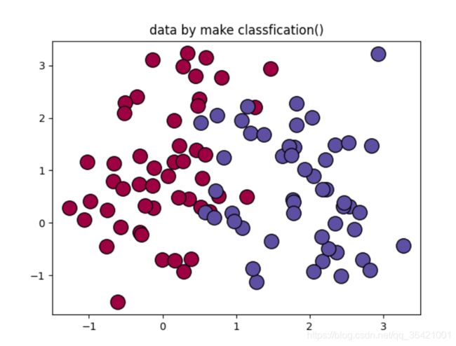
    def create_data(self):
        x, labels = make_classification(n_samples=100, n_features=2, n_redundant=0, n_informative=2, random_state=1,
                                        n_clusters_per_class=2)
        #labels=labels.reshape((-1,1))
        #画出数据分布图
        rng = np.random.RandomState(2)
        x += 2 * rng.uniform(size=x.shape)
        unique_label = set(labels)
        colors = plt.cm.Spectral(np.linspace(0, 1, len(unique_label)))
        for k, col in zip(unique_label, colors):
            x_k = x[labels == k]
            plt.plot(x_k[:, 0], x_k[:, 1], 'o', markerfacecolor=col, markeredgecolor='k', markersize=14)
        plt.title('data by make classfication()')
        # 对数据进行简单的训练集和测试集的划分
        offset = int(x.shape[0] * 0.9)
        x_train, y_train = x[:offset], labels[:offset]
        x_test, y_test = x[offset:], labels[offset:]
        y_train = y_train.reshape((-1, 1))
        y_test = y_test.reshape((-1, 1))
        print("x_train=", x_train.shape)
        print("x_test=", x_test.shape)
        print("y_train=", y_train.shape)
        print("y_test=", y_test.shape)
        return x_train, y_train, x_test, y_test

    # 最后我们定义个绘制模型决策边界的图形函数对训练结果进行可视化展示：
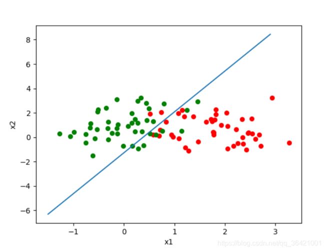
    def plot_logistic(self,x_train, y_train, params):
        n = x_train.shape[0]
        xcord1 = []
        ycord1 = []
        xcord2 = []
        ycord2 = []
        for i in range(n):
            if y_train[i] == 1:
                xcord1.append(x_train[i][0])
                ycord1.append(x_train[i][1])
            else:
                xcord2.append(x_train[i][0])
                ycord2.append(x_train[i][1])
        fig = plt.figure(2)
        ax = fig.add_subplot(111)
        ax.scatter(xcord1, ycord1, s=32, c='red')
        ax.scatter(xcord2, ycord2, s=32, c='green')
        x = np.arange(-1.5, 3, 0.1)
        y = (-params['b'] - params['w'][0] * x) / params['w'][1]#分界面
        ax.plot(x, y)
        plt.xlabel('x1')
        plt.ylabel('x2')
        plt.show()


if __name__=='__main__':
    model=logistic_regression()
    x_train,y_train,x_test,y_test=model.create_data()
    # 对训练集进行训练
    cost_list, params, grads = model.logistic_train(x_train, y_train, 0.01, 1000)
    print(params)
    #测试集数据进行测试
    y_prediction = model.predict(x_test, params)
    print(y_prediction)

    # 打印训练准确率
    y_train_pred = model.predict(x_train, params)
    accuracy_score_train = model.accuracy(y_train, y_train_pred)
    print('train accuracy is:',accuracy_score_train)
    # 打印测试准确率
    y_test_pred = model.predict(x_test, params)
    accuracy_score_test = model.accuracy(y_test, y_test_pred)
    print('test accuracy is:',accuracy_score_test)

    model.plot_logistic(x_train, y_train, params)