吴恩达机器学习ex1

#导入常用的库
import numpy as np
import pandas as pd
import matplotlib.pyplot as plt

1 单变量线性回归

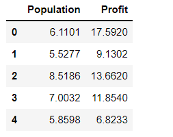
整个1的部分需要根据城市人口数量，预测开小吃店的利润数据在ex1data1.txt里，第一列是城市人口数量，第二列是该城市小吃店利润

关于单变量线性回归涉及到的公式：
(1)：h_theta(x)=theta₀+theta₁(x)
单变量线性回归需要求得的hypothesis

(2)：我们对上述公式进行转换，引入x₀=1，将X设置为[x₀,x₁]，对应的theta为[theta₀,theta₁]，上述公式转换为X和theta的内积

(3)：对应代价函数的公式如图所示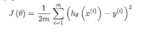
我们的目标就是求得最小的代价函数时theta向量

1.1 数据准备

读入数据然后展示

读数据使用read_csv()函数

# read_csv(filepath_or_buffer,sep,header,names)  
# filepath_or_buffer 文件的路径
# sep 字符串分隔符，默认为,
# header 整数，指定第几行为列名，如果没有指定默认为0
# names：列表，指定列名

path="./ex1data1.txt"
data = pd.read_csv(path, names=['Population', 'Profit'])
# head() 查看前五个，tail() 查看后五个 describe()查看各种描述
data.head()

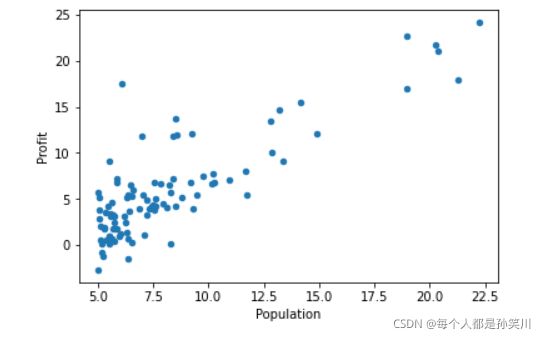
绘制散点图

data.plot(kind='scatter',x='Population',y='Profit')
# 或者可以使用
#data.plot.scatter('Population','Profit',label='Popultaion')
plt.show()

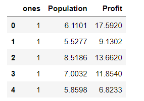
‘接下来根据上述公式理论(2)我们需要对数据集添加一列1
使用insert()函数即可

#data  的格式为DataFrame，插入可以使用insert进行插入
# insert(loc,column,value)
# loc,列索引；column；列的标签值；value；插入的值

data.insert(0,'ones',1)
data.head()

对数据进行切片，得到对应输入变量X和输出变量y，进行标签与数据的分离。

由于pandas读取的数据格式为DataFrame格式，我们之后处理矩阵需要使用numpy，所以将格式进行转换到ndarray，使用values()方法即可。

X=data.iloc[:,0:-1]
y=data.iloc[:,-1]
X=X.values
y=y.values
y=y.reshape(97,1)

1.2损失函数的定义

def computeCost(X,y,theta):
    inner=np.power(X@theta-y,2)
# 在这里之前使用的是X*theta一直报错，感谢up
    return np.sum(inner)/(2*len(X))

X为972,y为971，初始化theta为2*1向量

theta=np.zeros((2,1))
computeCost(X, y, theta)

1.3 梯度下降函数

def gradientDescent(X,y,theta,alpha,iters):
    costs=[]
    for i in range(iters):
        theta=theta-(X.T@(X@theta-y))*alpha/len(X)
        cost=computeCost(X,y,theta)
        costs.append(cost)
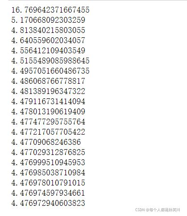
        if i % 100==0:
            print(cost)
    return theta,costs

iters=2000
alpha=0.02
theta,costs=gradientDescent(X,y,theta,alpha,iters)
# 可以看出已经收敛了

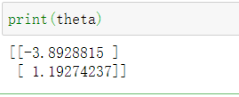
进行输出一下theta向量，便于之后与正规方程方法进行对比

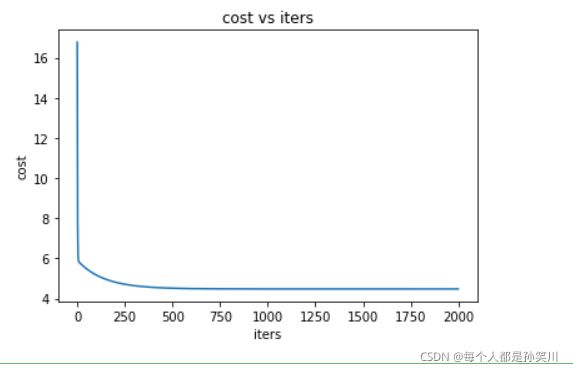
1.4 可视化损失函数

fig,ax=plt.subplots()
ax.plot(np.arange(iters),costs)
ax.set(xlabel='iters',
      ylabel='cost',
      title='cost vs iters')
plt.show()

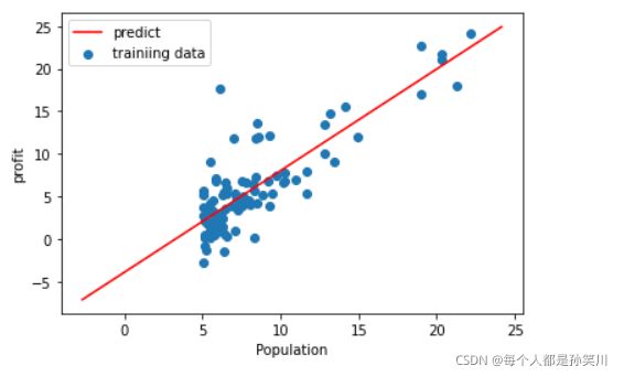
1.5 拟合函数可视化

x=np.linspace(y.min(),y.max(),100)
y_=theta[0,0]+theta[1,0]*x

fig,ax=plt.subplots()
ax.scatter(X[:,1],y,label='trainiing data')
ax.plot(x,y_,'r',label='predict')
ax.legend()
ax.set(xlabel='Population',
      ylabel='profit')
plt.show()

2 多变量线性回归

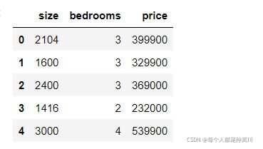
案例：假设你现在打算卖房子，想知道房子能卖多少钱？ 我们拥有房子面积和我是数量以及房子价格之间的对应数据：ex1data2.txt

2.1 读取文件

data=pd.read_csv('./ex1data2.txt',names=['size','bedrooms','price'])
data.head()

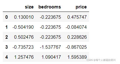
2.2 特征归一化

进行数据的预处理，特征归一化，也就是吴恩达老师所讲的特征缩放

目的： 消除特征值之间的量纲影响,各特征值处于同一数量级

提升模型的收敛速度

提升模型的精度

def nomalize_feature(data):
    return (data-data.mean())/data.std()

data=nomalize_feature(data)
data.head()

绘制散点图(不放图了)

data.plot.scatter('size','price',label='size')
plt.show()
data.plot.scatter('bedrooms','price',label='bedrooms')
plt.show()

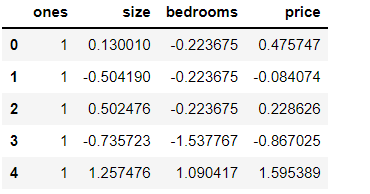
2.3 构造数据集

添加全为1的列

data.insert(0,'ones',1)
data.head()

切片

X=data.iloc[:,0:-1]
y=data.iloc[:,-1]
X=X.values
y=y.values
y=y.reshape(47,1)
X.shape,y.shape

2.4 损失函数的定义

def computeCost(X,y,theta):
    inner=np.power(X@theta-y,2)
    return np.sum(inner)/(2*len(X))

theta=np.zeros((3,1))
cost_init=computeCost(X,y,theta)
print(cost_init)

2.5 梯度下降函数

def gradientDescent(X,y,theta,alpha,iters,isprint=False):
    costs=[]
    for i in range(iters):
        theta=theta-(X.T@(X@theta-y))*alpha/len(X)
        cost=computeCost(X,y,theta)
        costs.append(cost)
        if i % 100==0:
            if isprint:
                print(cost)
    return theta,costs

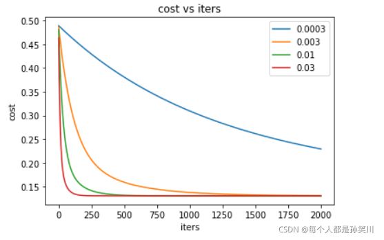
2.6 不同alpha下的效果

candidate_alpha=[0.0003,0.003,0.01,0.03]
iters=2000

fig,ax=plt.subplots()

for i in candidate_alpha:
    _,costs=gradientDescent(X,y,theta,i,iters)
    ax.plot(np.arange(iters),costs,label=i)
    ax.legend()

ax.set(xlabel='iters',
      ylabel='cost',
      title='cost vs iters')
plt.show()

3 正规方程

path="./ex1data1.txt"
data = pd.read_csv(path, names=['Population', 'Profit'])
data.insert(0,'ones',1)
X=data.iloc[:,0:-1]
y=data.iloc[:,-1]
X=X.values
y=y.values
y=y.reshape(97,1)

定义正规方程的函数

def NormalEquation(X,y):
    theta=np.linalg.inv(X.T@X)@X.T@y
    return theta

theta=NormalEquation(X,y)
print(theta)

可以看到正规方程的theta与上面单变量线性回归的theta差距不大，所以试验成功