支撑向量机 SVM

---

前言

---

一、SVM是什么？

SVM（support vector machine ） 支撑向量机
既可以解决分类问题也可以解决回归问题。

1、回顾逻辑回归

对于分类问题，比如逻辑回归，我们通常会使用一个决策边界来将不同的类别划分开来。

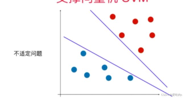
比如有不同的决策边界（称为不适定问题），如何找到最好的决策边界呢？逻辑回归是采用了损失函数，之后通过最小化损失函数来找到该决策边界。
那SVM是如何来寻找决策边界呢？

2、SVM求决策边界

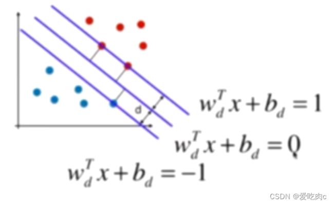
SVM是尝试寻找一个最优的决策边界：通过让两个类别中最近的样本距离该决策边界最远，同时该决策边界还能很好的划分该样本点。
这些离决策边界最近的点就称为支撑向量
不同类别的支撑向量之间的距离称为margin
SVM的目的就是要最大化margin

Hard Margin SVM 解决的是线性可分问题 决策边界可以没有错误的将样本点划分同时最大化了margin值
Soft Margin SVM 为了解决线性不可分问题

为了最大化margin，我们一定要先求出margin的数学表达式，之后求出其中的未知数，来最大化。
这也是我们机器学习尤其时参数学习中一个常用的思想：
将我们解决问题的思路变为了一个最优化问题，之后就是最优化目标函数

二、SVM最大化margin （hard margin svm）

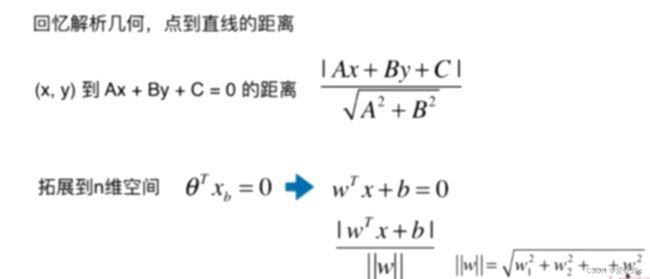
margin=2d 所以即最大化d 就需要列出d的数学形式 引出点到直线的距离

那我们就要求点到直线的距离
扩展到n维

在这里我们把二分类中的0和1改为1和-1这两类，只要区分开就行，没影响

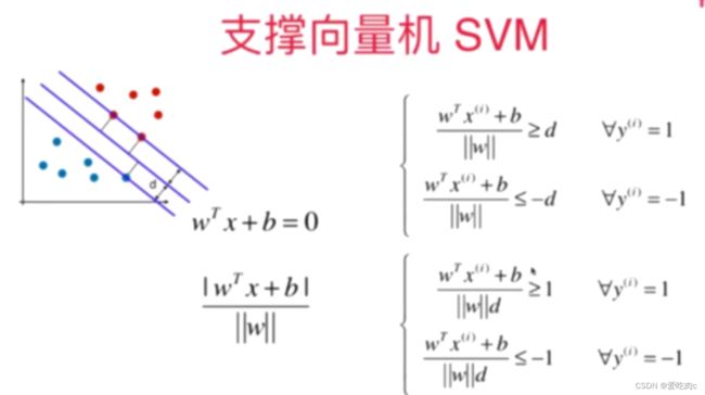
||w||d是一个常数，我们让wt 和b都除以这个常数 可以得到：

由于Wtx+b=0的右边部分为0，所以我们也可以让其同时除以||w||d
就变为统一的格式了

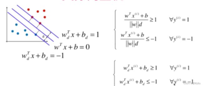
同时都用Wd和bd表示太过于麻烦，我们可以直接写为Wtx+b的形式
但这里的Wt与之前的Wt不同，这里是除以了||w||d.

同时我们可以将上下两类写成一个式子，就变成了如图所示的式子

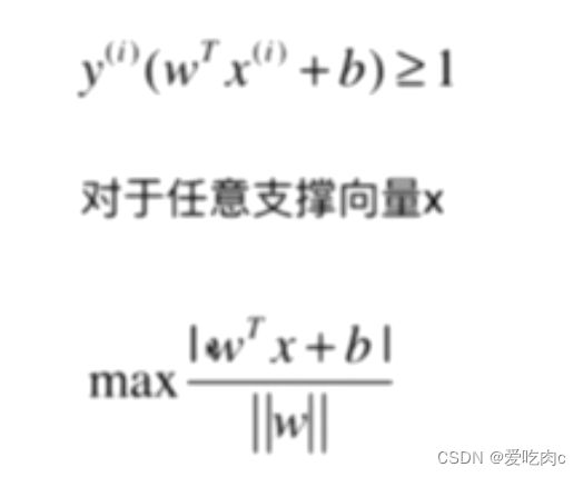
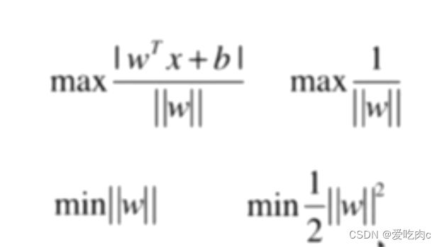
又由于支撑向量的直线的值都为1或-1，化简之后
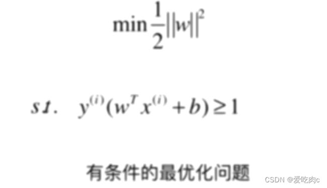
为了方便求导，写成平方

同时，这与我们之前讲的最优解问题不同，这是有条件的最优解问题，是局部的，而不是全局的，如果是全局的那么我们可以求导即可。但这里不行。

三、soft margin svm

1、引入

hard margin svm 首先要能正确分出不同类
比如这个图：

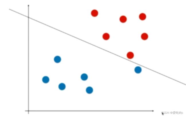
我们看这个图，觉得分类没问题，但是如果对于测试数据集，这个模型的泛化能力并不好，我们可以看到大多数蓝色点都在左下方，而这条直线却受了那一个蓝色极端点的影响。
又如：

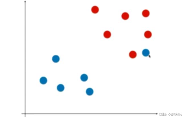
这是一个非线性问题，我们根本没有办法找到一条可以正确分类的决策边界。

所以此时就要引入soft margin svm。
允许模型有一定的容错能力。

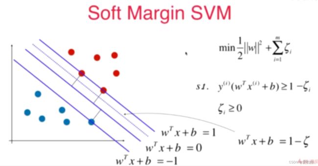
所以引入了一个参数，这使得模型有了一定的容错能力。如果是简单的hard margin svm 则要求所有的点都在margin外，在margin内部不得有样本点， 但是加上了这个系数之后，我们就使得margin内部也可以有少部分点，有了容错能力。相当于一个正则项。

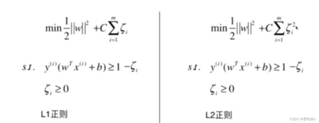
与以往的正则项相同，我们都需要在前面加上一个超参数，来平衡两者。
如果C越大，如果取一个极端值无穷大的话那我们就逼迫这这个参数为0，此时soft margin 就变为了 hard margin。
如果c越小，则我们的容错能力就越强。
更好的理解正则项，正则项可以是我们通过训练数据集来训练模型的时候，少受极端数据的影响。使模型能够有更好的泛化能力。

四、sklearn中的SVM

1、首先注意数据标准化

和KNN算法一样svm也涉及到距离，所以我们需要先将数据标准化。

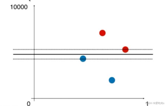
如图：如果两个样本特征量纲不同的话，像上边那幅图，就会受y轴这个样本特征的影响。
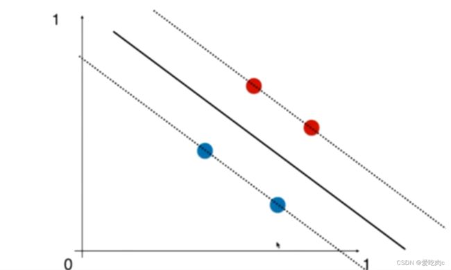
如果在相同的维度上，决策边界应该变成这样

2、sklearn中的SVM

SVM可以用来解决回归和分类问题

**svc天然的可以解决多分类问题，**所以它的系数coef_这些返回的都是二维矩阵，有多条直线，对应多条直线的系数

import numpy as np
import matplotlib.pyplot as plt
from sklearn import datasets
iris=datasets.load_iris()
x=iris.data
y=iris.target
x=x[y<2,:2] #先解决二分类问题 且为了可视化 我们先选择两个样本特征
y=y[y<2]
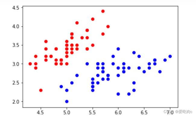
plt.scatter(x[y==0,0],x[y==0,1],color='r')
plt.scatter(x[y==1,0],x[y==1,1],color='b')
plt.show()

数据归一化

from sklearn.preprocessing import StandardScaler  #数据归一化
standsca=StandardScaler()
standsca.fit(x)
stand_x=standsca.transform(x)
from sklearn.svm import LinearSVC #解决分类问题的svc
svc=LinearSVC(C=1e9)#先让c很大，C很大，则相当于hard margin svm
svc.fit(stand_x,y)

绘制决策边界

def plot_decision_boundary(model,axis):
    x0,x1=np.meshgrid(
        np.linspace(axis[0],axis[1],int((axis[1]-axis[0]))*100).reshape(-1,1),
        np.linspace(axis[2],axis[3],int((axis[3]-axis[2]))*100).reshape(-1,1)
    )
    x_new=np.c_[x0.ravel(),x1.ravel()]
    y_predict=model.predict(x_new)
    zz=y_predict.reshape(x0.shape)
    from matplotlib.colors import ListedColormap
    custom_camp=ListedColormap(['#EF9A9A','#FFF59D','#90CAF9'])
    
    plt.contourf(x0,x1,zz,linewidth=5,camp=custom_camp)
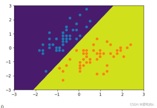
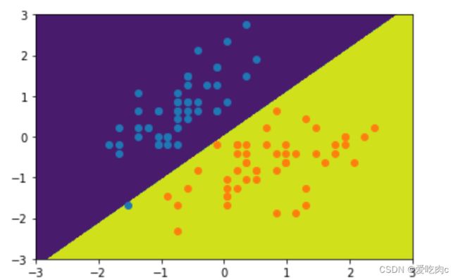
plot_decision_boundary(svc,[-3,3,-3,3])
plt.scatter(stand_x[y==0,0],stand_x[y==0,1])
plt.scatter(stand_x[y==1,0],stand_x[y==1,1])
plt.show()

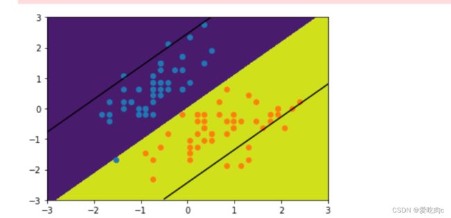
绘制带margin的决策边界 c很大时 相当于hard soft margin

def plot_svc_decision_boundary(model,axis):
    x0,x1=np.meshgrid(
        np.linspace(axis[0],axis[1],int((axis[1]-axis[0]))*100).reshape(-1,1),
        np.linspace(axis[2],axis[3],int((axis[3]-axis[2]))*100).reshape(-1,1)
    )
    x_new=np.c_[x0.ravel(),x1.ravel()]
    y_predict=model.predict(x_new)
    zz=y_predict.reshape(x0.shape)
    from matplotlib.colors import ListedColormap
    custom_camp=ListedColormap(['#EF9A9A','#FFF59D','#90CAF9'])
    
    plt.contourf(x0,x1,zz,linewidth=5,camp=custom_camp)
    w=model.coef_[0]
    b=model.intercept_[0]
    #w0*x0+w1*x1+b=0
    #->x1=-w0/w1*x0-b/w1  #根据x0就能绘制x1
    plot_x=np.linspace(axis[0],axis[1],200)
    up_y=-w[0]/w[1]*plot_x-b/w[1]+1/w[1] #上边那条margin
    down_y=-w[0]/w[1]*plot_x-b/w[1]-1/w[1] #下边那条
    up_index=(up_y>=axis[2])&(up_y<=axis[3])  #为了防止得到的y超出边界
    down_index=(down_y>=axis[2])&(down_y<=axis[3])
    plt.plot(plot_x[up_index],up_y[up_index],color='black')
    plt.plot(plot_x[down_index],down_y[down_index],color='black')

plot_svc_decision_boundary(svc,[-3,3,-3,3])
plt.scatter(stand_x[y==0,0],stand_x[y==0,1])
plt.scatter(stand_x[y==1,0],stand_x[y==1,1])
plt.show()

C很小时

svc2=LinearSVC(C=0.01)#先让c很大，C很大，则相当于hard margin svm
svc2.fit(stand_x,y)
y_predict=svc2.predict(stand_x)
plot_decision_boundary(svc2,[-3,3,-3,3])
plt.scatter(stand_x[y==0,0],stand_x[y==0,1])
plt.scatter(stand_x[y==1,0],stand_x[y==1,1])
plt.show()

plot_svc_decision_boundary(svc2,[-3,3,-3,3])
plt.scatter(stand_x[y==0,0],stand_x[y==0,1])
plt.scatter(stand_x[y==1,0],stand_x[y==1,1])
plt.show()

测试一下所有样本下的 不同的决策边界 对应的分类准确度
有兴趣的也可以测试一个极度偏斜的数据对应的精准率 召回率等指标

iris=datasets.load_iris()
x=iris.data
y=iris.target
from sklearn.model_selection import train_test_split
x_train,x_test,y_train,y_test=train_test_split(x,y,random_state=666)
from sklearn.preprocessing import StandardScaler  #数据归一化
standsca=StandardScaler()
standsca.fit(x_train)
stand_x_train=standsca.transform(x_train)
stand_x_test=standsca.transform(x_test)  #测试数据集 也要在训练数集得到的方差等数据上进行归一化
from sklearn.svm import LinearSVC #解决分类问题的svc
svc=LinearSVC(C=1e9)#先让c很大，C很大，则相当于hard margin svm
svc.fit(stand_x_train,y_train)
y_predict=svc.predict(stand_x_test)
svc.score(stand_x_test,y_predict)

1.0

svc2=LinearSVC(C=0.01)
svc2.fit(stand_x_train,y_train)
y2_predict=svc2.predict(stand_x_test)
svc.score(stand_x_test,y2_predict)

0.789…

五、使用SVM来解决非线性问题

1、使用多项式特征的SVM

import numpy as np
import  matplotlib.pyplot as plt
from sklearn import datasets
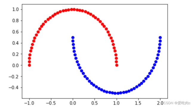
x,y=datasets.make_moons()
plt.scatter(x[y==0,0],x[y==0,1],color='r')
plt.scatter(x[y==1,0],x[y==1,1],color='b')
plt.show()

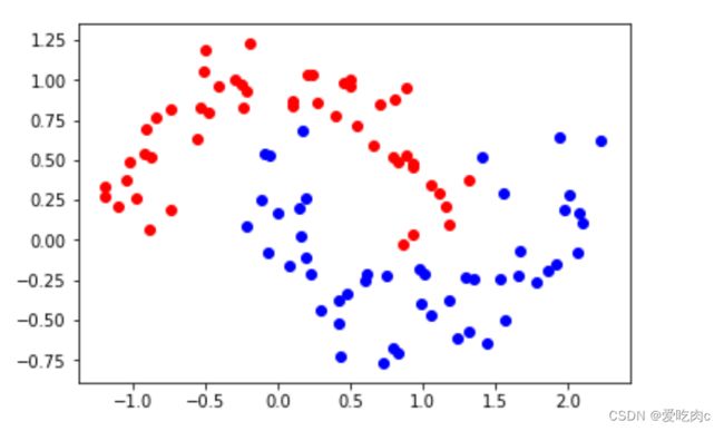
#添加噪声
x,y=datasets.make_moons(noise=0.15,random_state=666)
plt.scatter(x[y==0,0],x[y==0,1],color='r')
plt.scatter(x[y==1,0],x[y==1,1],color='b')
plt.show()

from sklearn.preprocessing import StandardScaler,PolynomialFeatures
from sklearn.pipeline import  Pipeline
from sklearn.svm import LinearSVC
def polysvm(degree,C=1.0):
    return Pipeline([
        ('poly',PolynomialFeatures(degree=degree)),
        ('std',StandardScaler()),
        ('svc',LinearSVC(C=C))
    ])
def plot_decision_boundary(model,axis):
    x0,x1=np.meshgrid(
        np.linspace(axis[0],axis[1],int((axis[1]-axis[0]))*100).reshape(-1,1),
        np.linspace(axis[2],axis[3],int((axis[3]-axis[2]))*100).reshape(-1,1)
    )
    x_new=np.c_[x0.ravel(),x1.ravel()]
    y_predict=model.predict(x_new)
    zz=y_predict.reshape(x0.shape)
    from matplotlib.colors import ListedColormap
    custom_camp=ListedColormap(['#EF9A9A','#FFF59D','#90CAF9'])
    
    plt.contourf(x0,x1,zz,linewidth=5,camp=custom_camp)
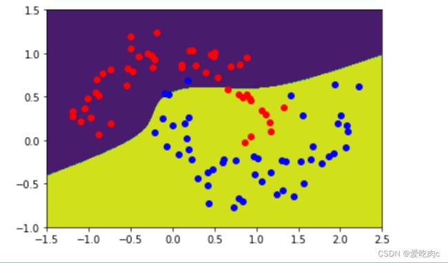
poly_svc=polysvm(degree=3)
poly_svc.fit(x,y)
plot_decision_boundary(poly_svc,[-1.5,2.5,-1.0,1.5])
plt.scatter(x[y==0,0],x[y==0,1],color='r')
plt.scatter(x[y==1,0],x[y==1,1],color='b')
plt.show()

2、使用多项式核函数的SVM

from sklearn.svm import SVC
def polykernelsvm(degree,C=1.0):
    return Pipeline([
        ('std',StandardScaler()),
        ('svc',SVC(kernel="poly",degree=degree,C=C))
    ])
poly_kernelsvc=polykernelsvm(degree=3)
poly_kernelsvc.fit(x,y)
plot_decision_boundary(poly_kernelsvc,[-1.5,2.5,-1.0,1.5])
plt.scatter(x[y==0,0],x[y==0,1],color='r')
plt.scatter(x[y==1,0],x[y==1,1],color='b')
plt.show()

总结

下篇文章讲解 核函数 高斯核函数等