Logistic回归(随机梯度上升算法)
梯度上升算法
def gradAscent(dataMatIn, classLabels):
    dataMatrix = np.mat(dataMatIn)                                        #转换成numpy的mat
    labelMat = np.mat(classLabels).transpose()                            #转换成numpy的mat,并进行转置
    m, n = np.shape(dataMatrix)                                            #返回dataMatrix的大小。m为行数,n为列数。
    alpha = 0.01                                                        #移动步长,也就是学习速率,控制更新的幅度。
    maxCycles = 500                                                        #最大迭代次数
    weights = np.ones((n,1))
    for k in range(maxCycles):
        h = sigmoid(dataMatrix * weights)                                #梯度上升矢量化公式
        error = labelMat - h
        weights = weights + alpha * dataMatrix.transpose() * error
    return weights.getA(),weights_array
随机梯度上升算法
def stocGradAscent1(dataMatrix, classLabels, numIter=150):
    m,n = np.shape(dataMatrix)                                                #返回dataMatrix的大小。m为行数,n为列数。
    weights = np.ones(n)                                                       #参数初始化
    for j in range(numIter):
        dataIndex = list(range(m))
        for i in range(m):
            alpha = 4/(1.0+j+i)+0.01                                            #降低alpha的大小,每次减小1/(j+i)。
            randIndex = int(random.uniform(0,len(dataIndex)))                #随机选取样本
            h = sigmoid(sum(dataMatrix[dataIndex[randIndex]]*weights))  #选择随机选取的一个样本,计算h
            error = classLabels[dataIndex[randIndex]] - h                           #计算误差
            weights = weights + alpha * error * dataMatrix[dataIndex[randIndex]]   #更新回归系数
            del(dataIndex[randIndex])                                         #删除已经使用的样本
    return weights
import matplotlib.pyplot as plt
import numpy as np
import random
def loadDataSet():
dataMat = [] # 创建数据列表
labelMat = [] # 创建标签列表
fr = open('testSet.txt') # 打开文件
for line in fr.readlines(): # 逐行读取
lineArr = line.strip().split() # 去回车,放入列表
dataMat.append([1.0, float(lineArr[0]), float(lineArr[1])]) # 添加数据
labelMat.append(int(lineArr[2])) # 添加标签
fr.close() # 关闭文件
return dataMat, labelMat # 返回
def sigmoid(inX):
return 1.0 / (1 + np.exp(-inX))
"""
函数说明:绘制数据集
Parameters:
weights - 权重参数数组
"""
def plotBestFit(weights):
dataMat, labelMat = loadDataSet() # 加载数据集
dataArr = np.array(dataMat) # 转换成numpy的array数组
n = np.shape(dataMat)[0] # 数据个数
xcord1 = []
ycord1 = [] # 正样本
xcord2 = []
ycord2 = [] # 负样本
for i in range(n): # 根据数据集标签进行分类
if int(labelMat[i]) == 1:
xcord1.append(dataArr[i, 1])
ycord1.append(dataArr[i, 2]) # 1为正样本
else:
xcord2.append(dataArr[i, 1])
ycord2.append(dataArr[i, 2]) # 0为负样本
fig = plt.figure()
ax = fig.add_subplot(111) # 添加subplot
ax.scatter(xcord1, ycord1, s=20, c='red', marker='s', alpha=.5) # 绘制正样本
ax.scatter(xcord2, ycord2, s=20, c='green', alpha=.5) # 绘制负样本
x = np.arange(-3.0, 3.0, 0.1)
y = (-weights[0] - weights[1] * x) / weights[2]
ax.plot(x, y)
plt.title('BestFit') # 绘制title
plt.xlabel('X1')
plt.ylabel('X2') # 绘制label
plt.show()
"""
函数说明:改进的随机梯度上升算法
Parameters:
dataMatrix - 数据数组
classLabels - 数据标签
numIter - 迭代次数
Returns:
weights - 求得的回归系数数组(最优参数)
"""
def stocGradAscent1(dataMatrix, classLabels, numIter=150):
m, n = np.shape(dataMatrix) # 返回dataMatrix的大小。m为行数,n为列数。
weights = np.ones(n) # 参数初始化
for j in range(numIter):
dataIndex = list(range(m))
for i in range(m):
alpha = 4 / (1.0 + j + i) + 0.01 # 降低alpha的大小,每次减小1/(j+i)。
randIndex = int(random.uniform(0, len(dataIndex))) # 随机选取样本
h = sigmoid(sum(dataMatrix[dataIndex[randIndex]] * weights)) # 选择随机选取的一个样本,计算h
error = classLabels[dataIndex[randIndex]] - h # 计算误差
weights = weights + alpha * error * dataMatrix[dataIndex[randIndex]] # 更新回归系数
del (dataIndex[randIndex]) # 删除已经使用的样本
return weights # 返回
def gradAscent(dataMatIn, classLabels):
dataMatrix = np.mat(dataMatIn) #转换成numpy的mat
labelMat = np.mat(classLabels).transpose() #转换成numpy的mat,并进行转置
m, n = np.shape(dataMatrix) #返回dataMatrix的大小。m为行数,n为列数。
alpha = 0.01 #移动步长,也就是学习速率,控制更新的幅度。
maxCycles = 500 #最大迭代次数
weights = np.ones((n,1))
weights_array = np.array([])
for k in range(maxCycles):
h = sigmoid(dataMatrix * weights) #梯度上升矢量化公式
error = labelMat - h
weights = weights + alpha * dataMatrix.transpose() * error
weights_array = np.append(weights_array,weights)
weights_array = weights_array.reshape(maxCycles,n)
return weights.getA(),weights_array #将矩阵转换为数组,并返回
if __name__ == '__main__':
dataMat, labelMat = loadDataSet()
weights = stocGradAscent1(np.array(dataMat), labelMat)
plotBestFit(weights)回归系数与迭代次数的关系
from matplotlib.font_manager import FontProperties
import matplotlib.pyplot as plt
import numpy as np
import random

"""
函数说明:加载数据

Parameters:
    无
Returns:
    dataMat - 数据列表
    labelMat - 标签列表
"""
def loadDataSet():
    dataMat = []                                                        #创建数据列表
    labelMat = []                                                        #创建标签列表
    fr = open('testSet.txt')                                            #打开文件
    for line in fr.readlines():                                            #逐行读取
        lineArr = line.strip().split()                                    #去回车,放入列表
        dataMat.append([1.0, float(lineArr[0]), float(lineArr[1])])        #添加数据
        labelMat.append(int(lineArr[2]))                                #添加标签
    fr.close()                                                            #关闭文件
    return dataMat, labelMat                                            #返回

def sigmoid(inX):
    return 1.0 / (1 + np.exp(-inX))

"""
函数说明:梯度上升算法

Parameters:
    dataMatIn - 数据集
    classLabels - 数据标签
Returns:
    weights.getA() - 求得的权重数组(最优参数)
    weights_array - 每次更新的回归系数
"""
def gradAscent(dataMatIn, classLabels):
    dataMatrix = np.mat(dataMatIn)                                        #转换成numpy的mat
    labelMat = np.mat(classLabels).transpose()                            #转换成numpy的mat,并进行转置
    m, n = np.shape(dataMatrix)                                            #返回dataMatrix的大小。m为行数,n为列数。
    alpha = 0.01                                                        #移动步长,也就是学习速率,控制更新的幅度。
    maxCycles = 500                                                        #最大迭代次数
    weights = np.ones((n,1))
    weights_array = np.array([])
    for k in range(maxCycles):
        h = sigmoid(dataMatrix * weights)                                #梯度上升矢量化公式
        error = labelMat - h
        weights = weights + alpha * dataMatrix.transpose() * error
        weights_array = np.append(weights_array,weights)
    weights_array = weights_array.reshape(maxCycles,n)
    return weights.getA(),weights_array                                    #将矩阵转换为数组,并返回

"""
函数说明:改进的随机梯度上升算法

Parameters:
    dataMatrix - 数据数组
    classLabels - 数据标签
    numIter - 迭代次数
Returns:
    weights - 求得的回归系数数组(最优参数)
    weights_array - 每次更新的回归系数
"""
def stocGradAscent1(dataMatrix, classLabels, numIter=150):
    m,n = np.shape(dataMatrix)                                                #返回dataMatrix的大小。m为行数,n为列数。
    weights = np.ones(n)                                                       #参数初始化
    weights_array = np.array([])                                            #存储每次更新的回归系数
    for j in range(numIter):
        dataIndex = list(range(m))
        for i in range(m):
            alpha = 4/(1.0+j+i)+0.01                                            #降低alpha的大小,每次减小1/(j+i)。
            randIndex = int(random.uniform(0,len(dataIndex)))                #随机选取样本
            h = sigmoid(sum(dataMatrix[dataIndex[randIndex]]*weights))          #选择随机选取的一个样本,计算h
            error = classLabels[dataIndex[randIndex]] - h                           #计算误差
            weights = weights + alpha * error * dataMatrix[dataIndex[randIndex]]   #更新回归系数
            weights_array = np.append(weights_array,weights,axis=0)         #添加回归系数到数组中
            del(dataIndex[randIndex])                                         #删除已经使用的样本
    weights_array = weights_array.reshape(numIter*m,n)                         #改变维度
    return weights,weights_array                                             #返回

"""
函数说明:绘制回归系数与迭代次数的关系

Parameters:
    weights_array1 - 回归系数数组1
    weights_array2 - 回归系数数组2
"""
def plotWeights(weights_array1,weights_array2):
    #设置汉字格式
    font = FontProperties(fname=r"c:\windows\fonts\simsun.ttc", size=14)
    #将fig画布分隔成1行1列,不共享x轴和y轴,fig画布的大小为(13,8)
    #当nrow=3,nclos=2时,代表fig画布被分为六个区域,axs[0][0]表示第一行第一列
    fig, axs = plt.subplots(nrows=3, ncols=2,sharex=False, sharey=False, figsize=(20,10))
    x1 = np.arange(0, len(weights_array1), 1)
    #绘制w0与迭代次数的关系
    axs[0][0].plot(x1,weights_array1[:,0])
    axs0_title_text = axs[0][0].set_title(u'梯度上升算法:回归系数与迭代次数关系',FontProperties=font)
    axs0_ylabel_text = axs[0][0].set_ylabel(u'W0',FontProperties=font)
    plt.setp(axs0_title_text, size=20, weight='bold', color='black')
    plt.setp(axs0_ylabel_text, size=20, weight='bold', color='black')
    #绘制w1与迭代次数的关系
    axs[1][0].plot(x1,weights_array1[:,1])
    axs1_ylabel_text = axs[1][0].set_ylabel(u'W1',FontProperties=font)
    plt.setp(axs1_ylabel_text, size=20, weight='bold', color='black')
    #绘制w2与迭代次数的关系
    axs[2][0].plot(x1,weights_array1[:,2])
    axs2_xlabel_text = axs[2][0].set_xlabel(u'迭代次数',FontProperties=font)
    axs2_ylabel_text = axs[2][0].set_ylabel(u'W2',FontProperties=font)
    plt.setp(axs2_xlabel_text, size=20, weight='bold', color='black')
    plt.setp(axs2_ylabel_text, size=20, weight='bold', color='black')


    x2 = np.arange(0, len(weights_array2), 1)
    #绘制w0与迭代次数的关系
    axs[0][1].plot(x2,weights_array2[:,0])
    axs0_title_text = axs[0][1].set_title(u'改进的随机梯度上升算法:回归系数与迭代次数关系',FontProperties=font)
    axs0_ylabel_text = axs[0][1].set_ylabel(u'W0',FontProperties=font)
    plt.setp(axs0_title_text, size=20, weight='bold', color='black')
    plt.setp(axs0_ylabel_text, size=20, weight='bold', color='black')
    #绘制w1与迭代次数的关系
    axs[1][1].plot(x2,weights_array2[:,1])
    axs1_ylabel_text = axs[1][1].set_ylabel(u'W1',FontProperties=font)
    plt.setp(axs1_ylabel_text, size=20, weight='bold', color='black')
    #绘制w2与迭代次数的关系
    axs[2][1].plot(x2,weights_array2[:,2])
    axs2_xlabel_text = axs[2][1].set_xlabel(u'迭代次数',FontProperties=font)
    axs2_ylabel_text = axs[2][1].set_ylabel(u'W1',FontProperties=font)
    plt.setp(axs2_xlabel_text, size=20, weight='bold', color='black')
    plt.setp(axs2_ylabel_text, size=20, weight='bold', color='black')

    plt.show()

if __name__ == '__main__':
    dataMat, labelMat = loadDataSet()
    weights1,weights_array1 = stocGradAscent1(np.array(dataMat), labelMat)

    weights2,weights_array2 = gradAscent(dataMat, labelMat)
    plotWeights(weights_array1, weights_array2)
由于改进的随机梯度上升算法,随机选取样本点,所以每次的运行结果是不同的。但是大体趋势是一样的。我们改进的随机梯度上升算法收敛效果更好。为什么这么说呢?让我们分析一下。我们一共有100个样本点,改进的随机梯度上升算法迭代次数为150。而上图显示15000次迭代次数的原因是,使用一次样本就更新一下回归系数。因此,迭代150次,相当于更新回归系数150*100=15000次。简而言之,迭代150次,更新1.5万次回归参数。从上图左侧的改进随机梯度上升算法回归效果中可以看出,其实在更新2000次回归系数的时候,已经收敛了。相当于遍历整个数据集20次的时候,回归系数已收敛。训练已完成。
再让我们看看上图右侧的梯度上升算法回归效果,梯度上升算法每次更新回归系数都要遍历整个数据集。从图中可以看出,当迭代次数为300多次的时候,回归系数才收敛。凑个整,就当它在遍历整个数据集300次的时候已经收敛好了。
没有对比就没有伤害,改进的随机梯度上升算法,在遍历数据集的第20次开始收敛。而梯度上升算法,在遍历数据集的第300次才开始收敛。想像一下,大量数据的情况下,谁更牛逼?
使用Sklearn构建Logistic回归分类器
实战
缺失值的处理
- 使用可用特征的均值来填补缺失值;
- 使用特殊值来填补缺失值,如-1;
- 忽略有缺失值的样本;
- 使用相似样本的均值添补缺失值;
- 使用另外的机器学习算法预测缺失值。
预处理数据做两件事:
- 如果测试集中一条数据的特征值已经确实,那么我们选择实数0来替换所有缺失值,因为本文使用Logistic回归。因此这样做不会影响回归系数的值。sigmoid(0)=0.5,即它对结果的预测不具有任何倾向性。
- 如果测试集中一条数据的类别标签已经缺失,那么我们将该类别数据丢弃,因为类别标签与特征不同,很难确定采用某个合适的值来替换。
sklearn.linear_model.LogisticRegression
参数说明如下:
- penalty:惩罚项,str类型,可选参数为l1和l2,默认为l2。用于指定惩罚项中使用的规范。newton-cg、sag和lbfgs求解算法只支持L2规范。L1G规范假设的是模型的参数满足拉普拉斯分布,L2假设的模型参数满足高斯分布,所谓的范式就是加上对参数的约束,使得模型更不会过拟合(overfit),但是如果要说是不是加了约束就会好,这个没有人能回答,只能说,加约束的情况下,理论上应该可以获得泛化能力更强的结果。
- dual:对偶或原始方法,bool类型,默认为False。对偶方法只用在求解线性多核(liblinear)的L2惩罚项上。当样本数量>样本特征的时候,dual通常设置为False。
- tol:停止求解的标准,float类型,默认为1e-4。就是求解到多少的时候,停止,认为已经求出最优解。
- c:正则化系数λ的倒数,float类型,默认为1.0。必须是正浮点型数。像SVM一样,越小的数值表示越强的正则化。
- fit_intercept:是否存在截距或偏差,bool类型,默认为True。
- intercept_scaling:仅在正则化项为"liblinear",且fit_intercept设置为True时有用。float类型,默认为1。
- class_weight:用于标示分类模型中各种类型的权重,可以是一个字典或者'balanced'字符串,默认为不输入,也就是不考虑权重,即为None。如果选择输入的话,可以选择balanced让类库自己计算类型权重,或者自己输入各个类型的权重。举个例子,比如对于0,1的二元模型,我们可以定义class_weight={0:0.9,1:0.1},这样类型0的权重为90%,而类型1的权重为10%。如果class_weight选择balanced,那么类库会根据训练样本量来计算权重。某种类型样本量越多,则权重越低,样本量越少,则权重越高。当class_weight为balanced时,类权重计算方法如下:n_samples / (n_classes * np.bincount(y))。n_samples为样本数,n_classes为类别数量,np.bincount(y)会输出每个类的样本数,例如y=[1,0,0,1,1],则np.bincount(y)=[2,3]。
- 那么class_weight有什么作用呢?
- 在分类模型中,我们经常会遇到两类问题:
- 1.第一种是误分类的代价很高。比如对合法用户和非法用户进行分类,将非法用户分类为合法用户的代价很高,我们宁愿将合法用户分类为非法用户,这时可以人工再甄别,但是却不愿将非法用户分类为合法用户。这时,我们可以适当提高非法用户的权重。
- 2. 第二种是样本是高度失衡的,比如我们有合法用户和非法用户的二元样本数据10000条,里面合法用户有9995条,非法用户只有5条,如果我们不考虑权重,则我们可以将所有的测试集都预测为合法用户,这样预测准确率理论上有99.95%,但是却没有任何意义。这时,我们可以选择balanced,让类库自动提高非法用户样本的权重。提高了某种分类的权重,相比不考虑权重,会有更多的样本分类划分到高权重的类别,从而可以解决上面两类问题。
- random_state:随机数种子,int类型,可选参数,默认为无,仅在正则化优化算法为sag,liblinear时有用。
- solver:优化算法选择参数,只有五个可选参数,即newton-cg,lbfgs,liblinear,sag,saga。默认为liblinear。solver参数决定了我们对逻辑回归损失函数的优化方法,有四种算法可以选择,分别是:
- liblinear:使用了开源的liblinear库实现,内部使用了坐标轴下降法来迭代优化损失函数。
- lbfgs:拟牛顿法的一种,利用损失函数二阶导数矩阵即海森矩阵来迭代优化损失函数。
- newton-cg:也是牛顿法家族的一种,利用损失函数二阶导数矩阵即海森矩阵来迭代优化损失函数。
- sag:即随机平均梯度下降,是梯度下降法的变种,和普通梯度下降法的区别是每次迭代仅仅用一部分的样本来计算梯度,适合于样本数据多的时候。
- saga:线性收敛的随机优化算法的的变重。
- 总结:
- liblinear适用于小数据集,而sag和saga适用于大数据集因为速度更快。
- 对于多分类问题,只有newton-cg,sag,saga和lbfgs能够处理多项损失,而liblinear受限于一对剩余(OvR)。啥意思,就是用liblinear的时候,如果是多分类问题,得先把一种类别作为一个类别,剩余的所有类别作为另外一个类别。一次类推,遍历所有类别,进行分类。
- newton-cg,sag和lbfgs这三种优化算法时都需要损失函数的一阶或者二阶连续导数,因此不能用于没有连续导数的L1正则化,只能用于L2正则化。而liblinear和saga通吃L1正则化和L2正则化。
- 同时,sag每次仅仅使用了部分样本进行梯度迭代,所以当样本量少的时候不要选择它,而如果样本量非常大,比如大于10万,sag是第一选择。但是sag不能用于L1正则化,所以当你有大量的样本,又需要L1正则化的话就要自己做取舍了。要么通过对样本采样来降低样本量,要么回到L2正则化。
- 从上面的描述,大家可能觉得,既然newton-cg, lbfgs和sag这么多限制,如果不是大样本,我们选择liblinear不就行了嘛!错,因为liblinear也有自己的弱点!我们知道,逻辑回归有二元逻辑回归和多元逻辑回归。对于多元逻辑回归常见的有one-vs-rest(OvR)和many-vs-many(MvM)两种。而MvM一般比OvR分类相对准确一些。郁闷的是liblinear只支持OvR,不支持MvM,这样如果我们需要相对精确的多元逻辑回归时,就不能选择liblinear了。也意味着如果我们需要相对精确的多元逻辑回归不能使用L1正则化了。
- max_iter:算法收敛最大迭代次数,int类型,默认为10。仅在正则化优化算法为newton-cg, sag和lbfgs才有用,算法收敛的最大迭代次数。
- multi_class:分类方式选择参数,str类型,可选参数为ovr和multinomial,默认为ovr。ovr即前面提到的one-vs-rest(OvR),而multinomial即前面提到的many-vs-many(MvM)。如果是二元逻辑回归,ovr和multinomial并没有任何区别,区别主要在多元逻辑回归上。
- OvR和MvM有什么不同?
- OvR的思想很简单,无论你是多少元逻辑回归,我们都可以看做二元逻辑回归。具体做法是,对于第K类的分类决策,我们把所有第K类的样本作为正例,除了第K类样本以外的所有样本都作为负例,然后在上面做二元逻辑回归,得到第K类的分类模型。其他类的分类模型获得以此类推。
- 而MvM则相对复杂,这里举MvM的特例one-vs-one(OvO)作讲解。如果模型有T类,我们每次在所有的T类样本里面选择两类样本出来,不妨记为T1类和T2类,把所有的输出为T1和T2的样本放在一起,把T1作为正例,T2作为负例,进行二元逻辑回归,得到模型参数。我们一共需要T(T-1)/2次分类。
- 可以看出OvR相对简单,但分类效果相对略差(这里指大多数样本分布情况,某些样本分布下OvR可能更好)。而MvM分类相对精确,但是分类速度没有OvR快。如果选择了ovr,则4种损失函数的优化方法liblinear,newton-cg,lbfgs和sag都可以选择。但是如果选择了multinomial,则只能选择newton-cg, lbfgs和sag了。
- verbose:日志冗长度,int类型。默认为0。就是不输出训练过程,1的时候偶尔输出结果,大于1,对于每个子模型都输出。
- warm_start:热启动参数,bool类型。默认为False。如果为True,则下一次训练是以追加树的形式进行(重新使用上一次的调用作为初始化)。
- n_jobs:并行数。int类型,默认为1。1的时候,用CPU的一个内核运行程序,2的时候,用CPU的2个内核运行程序。为-1的时候,用所有CPU的内核运行程序。
from sklearn.linear_model import LogisticRegression

"""
函数说明:使用Sklearn构建Logistic回归分类器
"""

def colicSklearn():
    frTrain = open('horseColicTraining.txt')  # 打开训练集
    frTest = open('horseColicTest.txt')  # 打开测试集
    trainingSet = []
    trainingLabels = []
    testSet = []
    testLabels = []
    for line in frTrain.readlines():
        currLine = line.strip().split('\t')
        lineArr = []
        for i in range(len(currLine) - 1):
            lineArr.append(float(currLine[i]))
        trainingSet.append(lineArr)
        trainingLabels.append(float(currLine[-1]))
    for line in frTest.readlines():
        currLine = line.strip().split('\t')
        lineArr = []
        for i in range(len(currLine) - 1):
            lineArr.append(float(currLine[i]))
        testSet.append(lineArr)
        testLabels.append(float(currLine[-1]))
    classifier = LogisticRegression(solver='liblinear', max_iter=10).fit(trainingSet, trainingLabels)
    test_accurcy = classifier.score(testSet, testLabels) * 100
    print('正确率:%f%%' % test_accurcy)

if __name__ == '__main__':
    colicSklearn()
示例2
from sklearn.linear_model import LogisticRegression
from sklearn.datasets import load_breast_cancer # 乳腺癌数据集
from sklearn.model_selection import train_test_split
from sklearn.metrics import accuracy_score
import numpy as np
import matplotlib.pyplot as plt
# 获得特征标签数据
data = load_breast_cancer()
X = data['data']
y = data['target']
# 分割训练姐测试集
X_train, X_test, y_train, y_test = train_test_split(X, y, test_size=0.3, random_state=1)
lr_l1 = LogisticRegression(penalty="l1", C=0.5, solver="liblinear")
lr_l2 = LogisticRegression(penalty="l2", C=0.5, solver="liblinear")
# 训练模型
lr_l1.fit(X_train, y_train)
lr_l2.fit(X_train, y_train)
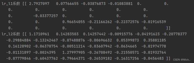
print('lr_l1系数',lr_l1.coef_)
print('lr_l2系数',lr_l2.coef_)
# 训练集表现
l1_train_predict = []
l2_train_predict = []
# 测试集表现
l1_test_predict = []
l2_test_predict = []
for c in np.linspace(0.01, 2, 50):
lr_l1 = LogisticRegression(penalty="l1", C=c, solver="liblinear", max_iter=10000)
lr_l2 = LogisticRegression(penalty='l2', C=c, solver='liblinear', max_iter=10000)
# 训练模型,记录L1正则化模型在训练集测试集上的表现
lr_l1.fit(X_train, y_train)
l1_train_predict.append(accuracy_score(lr_l1.predict(X_train), y_train))
l1_test_predict.append(accuracy_score(lr_l1.predict(X_test), y_test))
# 记录L2正则化模型的表现
lr_l2.fit(X_train, y_train)
l2_train_predict.append(accuracy_score(lr_l2.predict(X_train), y_train))
l2_test_predict.append(accuracy_score(lr_l2.predict(X_test), y_test))
data = [l1_train_predict, l2_train_predict, l1_test_predict, l2_test_predict]
label = ['l1_train', 'l2_train', 'l1_test', "l2_test"]
color = ['red', 'green', 'orange', 'blue']
plt.figure(figsize=(12, 6))
for i in range(4):
plt.plot(np.linspace(0.01, 2, 50), data[i], label=label[i], color=color[i])
plt.legend(loc="best")
plt.show()

多分类问题
from sklearn.linear_model import LogisticRegression
# 导入鸢尾花数据集
from sklearn.datasets import load_iris
from sklearn.model_selection import cross_val_score
iris = load_iris()
X = iris.data
y = iris.target
lr = LogisticRegression(C=0.5, penalty='l2', solver='sag', multi_class="auto", max_iter=2000)
score = cross_val_score(lr, X, y, cv=10).mean()
print(score)
参考文献
机器学习实战教程(七):Logistic回归实战篇之预测病马死亡率 (cuijiahua.com)