Python吴恩达深度学习作业11 -- 卷积神经网络的实现

逐步实现卷积神经网络

在此作业中，你将使用numpy实现卷积（CONV）和池化（POOL）层，包括正向传播和反向传播。

符号：

• 上标 $[l]$ 表示第 $l^{th}$ 层的对象.
  • 例如: $a^{[4]}$ 是 $4^{th}$ 层的激活. $W^{[5]}$ 和 $b^{[5]}$ 是 $5^{th}$ 层的参数。
• 上标 $(i)$ 表示第$i^{th}$个示例中的对象。
  • 示例：$x^{(i)}$是$i^{th}$个训练数据的输入。
• 下标$i$表示$i^{th}$的向量输入。
  • 示例：$a_i^{[l]}$表示$l$层中的$i^{th}$个激活，假设这是全连接层(FC)。
• $n_H$，$n_W$和$n_C$分别表示给定层的通道的高度，宽度和数量。如果要应用特定层$l$，则还可以写入$n_H^{[l]}$, $n_W^{[l]}$, $n_C^{[l]}$。
• $n_{H_{prev}}$, $n_{W_{prev}}$ 和 $n_{C_{prev}}$分别表示前一层的高度，宽度和通道数。如果引用特定层$l$，则也可以表示为$n_H^{[l-1]}$, $n_W^{[l-1]}$, $n_C^{[l-1]}$。

我们假设你已经熟悉numpy或者已经完成了之前的专业课程。那就开始吧！

1 安装包

让我们首先导入在作业过程中需要用到的包：

• numpy 是Python科学计算的基本包。
• matplotlib 是在Python中常用的绘制图形的库。
• np.random.seed（1）使所有随机函数调用保持一致。这将帮助我们为你的作品评分。

import numpy as np
import h5py
import matplotlib.pyplot as plt

%matplotlib inline
plt.rcParams['figure.figsize'] = (5.0, 4.0) # set default size of plots
plt.rcParams['image.interpolation'] = 'nearest'
plt.rcParams['image.cmap'] = 'gray'

%load_ext autoreload
%autoreload 2

np.random.seed(1)

2 作业大纲

你将实现构建卷积神经网络的需要的模块！要求实现的每个函数都有详细的说明，以帮助你完成所需的步骤：

• 卷积函数，包括：
  • 零填充
  • 卷积窗口
  • 正向卷积
  • 反向卷积（可选）
• 池化函数，包括：
  • 正向池化
  • 创建mask
  • 分配值
  • 反向池化（可选）

本笔记本将要求你使用 numpy从头开始实现这些函数。在下一本笔记本中，你将学习使用TensorFlow来实现：

注意，对于每个正向函数，都有其对应的反向等式。因此，在正向传播模块的每一步中，都将一些参数存储在缓存中。这些参数用于在反向传播时计算梯度。

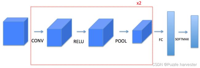
3 卷积神经网络

尽管编程框架可以方便使用卷积，但它们仍然是深度学习中最难理解的概念之一。卷积层将输入体积转换为不同大小的输出体积，如下所示。

在这一部分，你将构建卷积层的每一步。首先实现两个辅助函数：一个用于零填充，另一个用于计算卷积函数本身。

3.1 零填充

零填充将在图像的边界周围添加零：

图像（3个通道，RGB），填充2次。

填充的主要好处有：

• 允许使用CONV层而不必缩小其高度和宽度。这对于构建更深的网络很重要，因为高度/宽度会随着更深的层而缩小。一个重要、特殊的例子是"same"卷积，其中高度/宽度在一层之后被精确保留。
• 有助于我们将更多信息保留在图像边缘。如果不进行填充，下一层的一部分值将会受到图像边缘像素的干扰。

练习：实现以下函数，该功能将使用零填充处理一个批次X的所有图像数据。使用np.pad()。注意，如果要填充维度为$(5,5,5,5,5)$的数组"a",则第二维的填充为pad = 1，第四维的填充为pad = 3，其余为pad = 0，你可以这样做：

a = np.pad(a, ((0,0), (1,1), (0,0), (3,3), (0,0)), 'constant', constant_values = (..,..))

def zero_pad(X, pad):
    X_pad = np.pad(X, ((0,0), (pad, pad), (pad, pad), (0, 0)), 'constant', constant_values=0)
    
    return X_pad

np.random.seed(1)
x = np.random.randn(4, 3, 3, 2)
x_pad = zero_pad(x, 2)
print ("x.shape =", x.shape)
print ("x_pad.shape =", x_pad.shape)
print ("x[1,1] =", x[1,1])
print ("x_pad[1,1] =", x_pad[1,1])

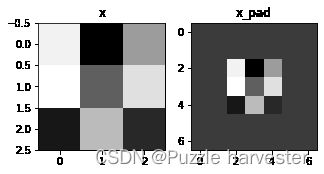
fig, axarr = plt.subplots(1, 2)
axarr[0].set_title('x')
axarr[0].imshow(x[0,:,:,0])
axarr[1].set_title('x_pad')
axarr[1].imshow(x_pad[0,:,:,0])

x.shape = (4, 3, 3, 2)
x_pad.shape = (4, 7, 7, 2)
x[1,1] = [[ 0.90085595 -0.68372786]
 [-0.12289023 -0.93576943]
 [-0.26788808  0.53035547]]
x_pad[1,1] = [[0. 0.]
 [0. 0.]
 [0. 0.]
 [0. 0.]
 [0. 0.]
 [0. 0.]
 [0. 0.]]

3.2 卷积的单个步骤

在这一部分中，实现卷积的单个步骤，其中将滤波器（卷积核）应用于输入的单个位置。这将用于构建卷积单元，该卷积单元：

• 占用输入体积
• 在输入的每个位置都应用滤波器
• 输出另一个体积（通常大小不同）
  

图2：卷积操作

滤波器大小为$2\times 2$，步幅为1（步幅 = 每次滑动窗口的数量）

在计算机视觉应用中，左侧矩阵中的每个值都对应一个像素值，我们将$3\times 3$滤波器与图像进行卷积操作，首先将滤波器元素的值与原始矩阵相乘，然后将它们相加。在练习的第一步中，你将实现卷积的单个步骤，相对于仅对一个位置应用滤波器以获得单个实值输出。

在本笔记本的后面，你将应用此函数于输入的多个位置以实现完整的卷积运算。

练习：实现conv_single_step()。

def conv_single_step(a_slice_prev, W, b):
    s = np.multiply(a_slice_prev, W) + b
    Z = np.sum(s)
    
    return Z

np.random.seed(1)
a_slice_prev = np.random.randn(4, 4, 3)
W = np.random.randn(4, 4, 3)
b = np.random.randn(1, 1, 1)

Z = conv_single_step(a_slice_prev, W, b)
print("Z =", Z)

Z = -23.16021220252078

3.3 卷积神经网络–正向传递

在正向传递中，你将使用多个滤波器对输入进行卷积。每个“卷积”都会输出一个2D矩阵。然后，你将堆叠这些输出以获得3：

练习：实现以下函数，使用滤波器W卷积输入A_prev。此函数将上一层的激活输出（对于一批m个输入）A_prev作为输入，F表示滤波器/权重（W）和偏置向量（b），其中每个滤波器都有自己的（单个）偏置。最后，你还可以访问包含stride和padding的超参数字典。

提示：

1. 要在矩阵"a_prev"(5,5,3)的左上角选择一个$2\times 2$切片，请执行以下操作：

a_slice_prev = a_prev[0:2,0:2,:]

使用定义的start/end索引定义a_slice_prev时将非常有用。

2. 要定义a_slice，你需要首先定义其角点vert_start,vert_end，horiz_strat和horiz_end。该图可能有助于你找到如何在下面的代码中使用h,w,f和s定义每个角。
   

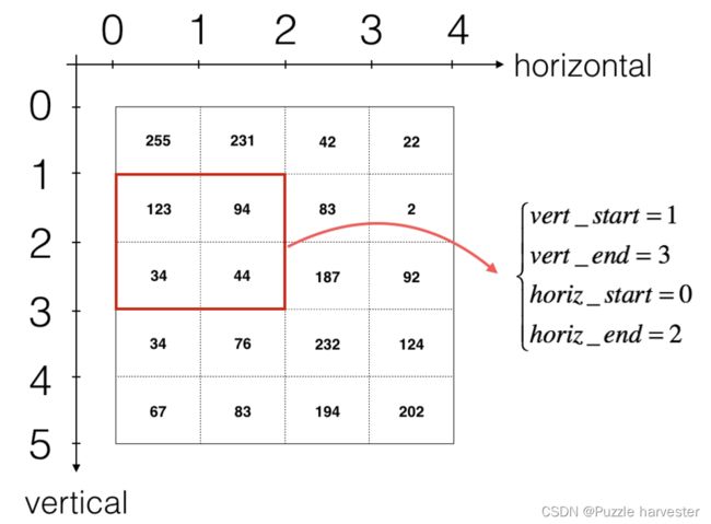
图3：使用垂直和水平的start/end（$2\times 2$滤波器）定义切片

该图仅显示一个通道。

提醒：

卷积的输出维度与输入维度相关公式为：
$$n_H=\lfloor \frac{n_{H_{prev}}-f+2\times pad}{stride}\rfloor +1$$
$$n_W=\lfloor \frac{n_{W_{prev}}-f+2\times pad}{stride}\rfloor +1$$
$$n_C=\text{number of filters used in the convolution}$$
对于此作业，我们不必考虑向量化，只使用for循环实现所有函数。

def conv_forward(A_prev, W, b, hparameters):
    
    (m, n_H_prev, n_W_prev, n_C_prev) = A_prev.shape
    
    (f, f, n_C_prev, n_C) = W.shape
    
    stride = hparameters['stride']
    pad = hparameters['pad']
    
    n_H = 1 + int((n_H_prev + 2 * pad - f) / stride)
    n_W = 1 + int((n_W_prev + 2 * pad - f) / stride)
    
    Z = np.zeros((m, n_H, n_W, n_C))
    
    A_prev_pad = zero_pad(A_prev, pad)
    
    for i in range(m):
        a_prev_pad = A_prev_pad[i]
        for h in range(n_H):
            for w in range(n_W):
                for c in range(n_C):
                    # 找到当前“切片”的角
                    vert_start = h * stride
                    vert_end = vert_start + f
                    horiz_start = w * stride
                    horiz_end = horiz_start + f
                    
                    # 使用边角来定义a_prev_pad的(3D)切片(参见单元格上方的提示)。
                    a_slice_prev = a_prev_pad[vert_start:vert_end, horiz_start:horiz_end, :]
                    
                    # 将(3D)切片与正确的滤波器W和偏置b进行卷积，得到一个输出神经元。
                    Z[i, h, w, c] = np.sum(np.multiply(a_slice_prev, W[:, :, :, c]) + b[:, :, :, c])
                    
    assert(Z.shape == (m, n_H, n_W, n_C))
    
    cache = (A_prev, W, b, hparameters)
                    
    return Z, cache       

np.random.seed(1)
A_prev = np.random.randn(10,4,4,3)
W = np.random.randn(2,2,3,8)
b = np.random.randn(1,1,1,8)
hparameters = {"pad" : 2,
               "stride": 1}

Z, cache_conv = conv_forward(A_prev, W, b, hparameters)
print("Z's mean =", np.mean(Z))
print("cache_conv[0][1][2][3] =", cache_conv[0][1][2][3])

Z's mean = 0.15585932488906465
cache_conv[0][1][2][3] = [-0.20075807  0.18656139  0.41005165]

最后，CONV层还应包含一个激活，此情况下，我们将添加以下代码行：

# Convolve the window to get back one output neuron  
Z[i, h, w, c] = ...  
# Apply activation  
A[i, h, w, c] = activation(Z[i, h, w, c])

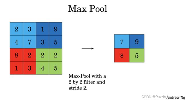
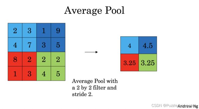
4 池化层

池化（POOL）层减少了输入的高度和宽度。它有助于减少计算量，而且可以使特征检测器在输入中的位置保持不变。池化层有两种：

• 最大池化：在输入上滑动$(f,f)$窗口，并将窗口的最大值存储在输出中。
• 平均池化：在输入上滑动$(f,f)$窗口，并将窗口的平均值存储在输出中。
  

这些池化层没有用于反向传播的参数。但是，它们具有超参数，例如窗口大小$f$，它指定了你要计算最大值或平均值的窗口的高度和宽度。

4.1 正向池化

现在，你将在同一函数中实现最大池化和平均池化。

练习：实现池化层的正向传播。请遵循下述提示。

提示：
由于没有填充，因此将池化的输出维度绑定到输入维度的公式：
$$n_H=\lfloor \frac{n_{H_{prev}}-f}{stride}\rfloor +1$$
$$n_W=\lfloor \frac{n_{W_{prev}}-f}{stride}\rfloor +1$$
$$n_C=n_{C_{prev}}$$

def pool_forward(A_prev, hparameters, mode = "max"):
    (m, n_H_prev, n_W_prev, n_C_prev) = A_prev.shape
    
    f = hparameters["f"]
    stride = hparameters["stride"]
    
    n_H = int(1 + (n_H_prev - f) / stride)
    n_W = int(1 + (n_W_prev - f) / stride)
    n_C = n_C_prev
    
    A = np.zeros((m, n_H, n_W, n_C))
    
    for i in range(m): # 样例数
        for h in range(n_H): # 在输出量的纵轴上循环
            for w in range(n_W): # 在输出量的横轴上循环
                for c in range(n_C):
                    # Step1:找切片
                    vert_start = h * stride
                    vert_end = vert_start + f
                    horiz_start = w * stride
                    horiz_end = horiz_start + f
                    
                    # Step2:使用角来定义A_prev的第i个训练示例的当前切片，通道c。
                    a_prev_slice = A_prev[i, vert_start:vert_end, horiz_start:horiz_end, c]
                    
                    # Step3:计算片上的池操作。使用if语句区分模式。使用np.max / np.mean。
                    if mode == "max":
                        A[i, h, w, c] = np.max(a_prev_slice)
                    elif mode == "average":
                        A[i, h, w, c] = np.mean(a_prev_slice)
    cache = (A_prev, hparameters)
    assert(A.shape == (m, n_H, n_W, n_C))
    
    return A, cache

np.random.seed(1)
A_prev = np.random.randn(2, 4, 4, 3)
hparameters = {"stride" : 1, "f": 4}

A, cache = pool_forward(A_prev, hparameters)
print("mode = max")
print("A =", A)
print()
A, cache = pool_forward(A_prev, hparameters, mode = "average")
print("mode = average")
print("A =", A)

mode = max
A = [[[[1.74481176 1.6924546  2.10025514]]]


 [[[1.19891788 1.51981682 2.18557541]]]]

mode = average
A = [[[[-0.09498456  0.11180064 -0.14263511]]]


 [[[-0.09525108  0.28325018  0.33035185]]]]

5 卷积神经网络中的反向传播

在深度学习框架中，你只需要实现正向传播，该框架就可以处理反向传播，因此大多数深度学习工程师不需要理会反向传播的细节。卷积网络的反向传播很复杂。但是，如果你愿意，可以在笔记本的此可选部分中进行操作，以了解卷积网络中反向传播的原理。

在较早的课程中，当你实现了一个简单的（全连接）神经网络时，你就使用了反向传播来计算损失的导数以更新参数。类似地，在卷积神经网络中，你可以计算损失的导数以更新参数。反向传播方程并非不重要，即使我们在课程中并未导出它们，但下面简要介绍了过程。

5.1 卷积层的反向传播

让我们从实现CONV层的反向传播开始。

5.1.1 计算 dA：

这是用于针对特定滤波器$W_c$的损失和给定训练示例计算$dA$的公式：
$$dA+=\sum _{h=0}^{n_H}\sum _{w=0}^{n_W}{W}_c\times d{Z}_{hw}\text{\hspace{1em}(1)}$$

其中$W_c$是一个滤波器，$d{Z}_{hw}$是一个标量，相对于第h行和第w列的conv层Z的输出的梯度的损失。请注意，每次更新dA时，我们都会将相同的滤波器$W_c$乘以不同的$dZ$。我们这样做主要是因为在计算正向传播时，每个滤波器都由不同的a_slice进行点乘和求和。因此，在为dA计算backprop时，我们只是加上所有a_slices的梯度。

在适当的for循环内，此公式转换为：

da_prev_pad[vert_start:vert_end, horiz_start:horiz_end, :] += W[:,:,:,c] * dZ[i, h, w, c]

5.1.2 计算 dW：

这是用于针对损失计算$d{W}_c$的公式（$d{W}_c$是一个滤波器的导数）：
$$d{W}_c+=\sum _{h=0}^{n_H}\sum _{w=0}^{n_W}{a}_{slice}\times d{Z}_{hw}\text{\hspace{1em}(2)}$$
其中$a_{slice}$对应于用于生成激活$Z_{ij}$的切片，最终我们得到$W$相对于该切片的梯度。由于它是相同的$W$，因此我们将所有这些梯度加起来即可得到$dW$。

在适当的for循环内，此公式转换为：

dW[:,:,:,c] += a_slice * dZ[i, h, w, c]

5.1.3 计算 db：

这是用于某个滤波器$W_c$的损失计算$db$的公式：
$$db=\sum _h\sum _{w}d{Z}_{hw}\text{\hspace{1em}(3)}$$
正如你先前在基本神经网络中所见，db是通过将$dZ$相加得出的。在这种情况下，你只需要对转换输出（Z）相对于损失的所有梯度求和。

在适当的for循环内，此公式转换为：

db[:,:,:,c] += dZ[i, h, w, c]

练习：在下面实现conv_backward函数。你应该总结所有训练数据，滤波器，高度和宽度。然后，你应该使用上面的公式1、2和3计算导数。

def conv_backward(dZ, cache):
    """
    Implement the backward propagation for a convolution function
    
    Arguments:
    dZ -- gradient of the cost with respect to the output of the conv layer (Z), numpy array of shape (m, n_H, n_W, n_C)
    cache -- cache of values needed for the conv_backward(), output of conv_forward()
    
    Returns:
    dA_prev -- gradient of the cost with respect to the input of the conv layer (A_prev),
               numpy array of shape (m, n_H_prev, n_W_prev, n_C_prev)
    dW -- gradient of the cost with respect to the weights of the conv layer (W)
          numpy array of shape (f, f, n_C_prev, n_C)
    db -- gradient of the cost with respect to the biases of the conv layer (b)
          numpy array of shape (1, 1, 1, n_C)
    """
    
    ### START CODE HERE ###
    # Retrieve information from "cache"
    (A_prev, W, b, hparameters) = cache
    
    # Retrieve dimensions from A_prev's shape
    (m, n_H_prev, n_W_prev, n_C_prev) = A_prev.shape
    
    # Retrieve dimensions from W's shape
    (f, f, n_C_prev, n_C) = W.shape
    
    # Retrieve information from "hparameters"
    stride = hparameters['stride']
    pad = hparameters['pad']
    
    # Retrieve dimensions from dZ's shape
    (m, n_H, n_W, n_C) = dZ.shape
    
    # Initialize dA_prev, dW, db with the correct shapes
    dA_prev = np.zeros((m, n_H_prev, n_W_prev, n_C_prev))                           
    dW = np.zeros((f, f, n_C_prev, n_C))
    db = np.zeros((1, 1, 1, n_C))

    # Pad A_prev and dA_prev
    A_prev_pad = zero_pad(A_prev, pad)
    dA_prev_pad = zero_pad(dA_prev, pad)
    
    for i in range(m):                       # loop over the training examples
        
        # select ith training example from A_prev_pad and dA_prev_pad
        a_prev_pad = A_prev_pad[i]
        da_prev_pad = dA_prev_pad[i]
        
        for h in range(n_H):                   # loop over vertical axis of the output volume
            for w in range(n_W):               # loop over horizontal axis of the output volume
                for c in range(n_C):           # loop over the channels of the output volume
                    
                    # Find the corners of the current "slice"
                    vert_start = h * stride
                    vert_end = vert_start + f
                    horiz_start = w * stride
                    horiz_end = horiz_start + f
                    
                    # Use the corners to define the slice from a_prev_pad
                    a_slice = a_prev_pad[vert_start:vert_end, horiz_start:horiz_end, :]

                    # Update gradients for the window and the filter's parameters using the code formulas given above
                    da_prev_pad[vert_start:vert_end, horiz_start:horiz_end, :] += W[:,:,:,c] * dZ[i, h, w, c]
                    dW[:,:,:,c] += a_slice * dZ[i, h, w, c]
                    db[:,:,:,c] += dZ[i, h, w, c]
                    
        # Set the ith training example's dA_prev to the unpaded da_prev_pad (Hint: use X[pad:-pad, pad:-pad, :])
        dA_prev[i, :, :, :] = dA_prev_pad[i, pad:-pad, pad:-pad, :]
    ### END CODE HERE ###
    
    # Making sure your output shape is correct
    assert(dA_prev.shape == (m, n_H_prev, n_W_prev, n_C_prev))
    
    return dA_prev, dW, db

np.random.seed(1)
dA, dW, db = conv_backward(Z, cache_conv)
print("dA_mean =", np.mean(dA))
print("dW_mean =", np.mean(dW))
print("db_mean =", np.mean(db))

dA_mean = 9.608990675868995
dW_mean = 10.581741275547566
db_mean = 76.37106919563735

5.2 池化层–反向传播

接下来，让我们从MAX-POOL层开始实现池化层的反向传播。即使池化层没有用于反向传播更新的参数，你仍需要通过池化层对梯度进行反向传播，以便计算池化层之前的层的梯度。

5.2.1 最大池化–反向传播

在进入池化层的反向传播之前，首先构建一个名为create_mask_from_window()的辅助函数，该函数将执行以下操作：
$$X=\left[\begin{array}{ccc}1& & 3\\ 4& & 2\end{array}\right]\to M=\left[\begin{array}{ccc}0& & 0\\ 1& & 0\end{array}\right]\text{\hspace{1em}(4)}$$
此函数创建一个“掩码”矩阵，该矩阵追踪矩阵的最大值。True（1）表示最大值在X中的位置，其他条目为False（0）。稍后你将看到，平均池的反向传播与此相似，但是使用了不同的掩码。

练习：实现create_mask_from_window（）。此函数将有助于反向池化。

提示：

• [np.max（）]（）可能会有所帮助。它计算一个数组的最大值。
• 如果有一个矩阵X和一个标量x：A =（X == x）将返回与X大小相同的矩阵A，从而：

A[i,j] = True if X[i,j] = x  
A[i,j] = False if X[i,j] != x

• 此处无需考虑矩阵中有多个最大值的情况。

def create_mask_from_window(x):
    """
    Creates a mask from an input matrix x, to identify the max entry of x.
    
    Arguments:
    x -- Array of shape (f, f)
    
    Returns:
    mask -- Array of the same shape as window, contains a True at the position corresponding to the max entry of x.
    """
    
    ### START CODE HERE ### (≈1 line)
    mask = (x == np.max(x))
    ### END CODE HERE ###
    
    return mask

np.random.seed(1)
x = np.random.randn(2,3)
mask = create_mask_from_window(x)
print('x = ', x)
print("mask = ", mask)

x =  [[ 1.62434536 -0.61175641 -0.52817175]
 [-1.07296862  0.86540763 -2.3015387 ]]
mask =  [[ True False False]
 [False False False]]

为什么我们要追踪最大值的位置？因为这是最终影响输出的输入值，也影响了损失。 反向传播算法是根据损失计算梯度的，因此影响最终损失的任何事物都应具有非零的梯度。因此，反向传播将使梯度“传播”回影响损失的特定输入值。

5.2.2 平均池化–反向传播

在最大池化中，对于每个输入窗口，输出上的所有“影响”都来自单个输入值，即最大值。在平均池化中，输入窗口的每个元素对输出的影响均相同 因此，要实现反向传播，你现在将实现一个反映此点的辅助函数。

例如，如果我们使用2x2滤波器在正向传播中进行平均池化，那么用于反向传播的掩码将如下所示：
$$dZ=1\to dZ=\left[\begin{array}{ccc}1/4& & 1/4\\ 1/4& & 1/4\end{array}\right]\text{\hspace{1em}(5)}$$
这意味着矩阵$dZ$中的每个位置对输出的贡献均等，因为在正向传播中，我们取平均值。

练习：实现以下函数，以通过维度矩阵平均分配值dz。 提示

def distribute_value(dz, shape):
    """
    Distributes the input value in the matrix of dimension shape
    
    Arguments:
    dz -- input scalar
    shape -- the shape (n_H, n_W) of the output matrix for which we want to distribute the value of dz
    
    Returns:
    a -- Array of size (n_H, n_W) for which we distributed the value of dz
    """
    
    ### START CODE HERE ###
    # Retrieve dimensions from shape (≈1 line)
    (n_H, n_W) = shape
    
    # Compute the value to distribute on the matrix (≈1 line)
    average = dz / (n_H * n_W)
    
    # Create a matrix where every entry is the "average" value (≈1 line)
    a = np.ones(shape) * average
    ### END CODE HERE ###
    
    return a

a = distribute_value(2, (2,2))
print('distributed value =', a)

distributed value = [[0.5 0.5]
 [0.5 0.5]]

5.2.3 组合：反向池化

现在，你准备好了在池化层上计算反向传播所需的一切。

练习：在两种模式（“max"和"average”）都实现“pool_backward”功能。再次使用4个for循环（遍历训练数据，高度，宽度和通道）。使用 if/elif语句来查看模式是否等于’max’或’average’。如果等于’average’ ，则应使用上面实现的distribute_value()函数创建与 a_slice维度相同的矩阵。此外，模式等于’max’时，你将使用 create_mask_from_window()创建一个掩码，并将其乘以相应的dZ值。

def pool_backward(dA, cache, mode = "max"):
    """
    Implements the backward pass of the pooling layer
    
    Arguments:
    dA -- gradient of cost with respect to the output of the pooling layer, same shape as A
    cache -- cache output from the forward pass of the pooling layer, contains the layer's input and hparameters 
    mode -- the pooling mode you would like to use, defined as a string ("max" or "average")
    
    Returns:
    dA_prev -- gradient of cost with respect to the input of the pooling layer, same shape as A_prev
    """
    
    ### START CODE HERE ###
    
    # Retrieve information from cache (≈1 line)
    (A_prev, hparameters) = cache
    
    # Retrieve hyperparameters from "hparameters" (≈2 lines)
    stride = hparameters['stride']
    f = hparameters['f']
    
    # Retrieve dimensions from A_prev's shape and dA's shape (≈2 lines)
    m, n_H_prev, n_W_prev, n_C_prev = A_prev.shape
    m, n_H, n_W, n_C = dA.shape
    
    # Initialize dA_prev with zeros (≈1 line)
    dA_prev = np.zeros_like(A_prev)
    
    for i in range(m):                       # loop over the training examples
        
        # select training example from A_prev (≈1 line)
        a_prev = A_prev[i]
        
        for h in range(n_H):                   # loop on the vertical axis
            for w in range(n_W):               # loop on the horizontal axis
                for c in range(n_C):           # loop over the channels (depth)
                    
                    # Find the corners of the current "slice" (≈4 lines)
                    vert_start = h * stride
                    vert_end = vert_start + f
                    horiz_start = w * stride
                    horiz_end = horiz_start + f
                    
                    # Compute the backward propagation in both modes.
                    if mode == "max":
                        
                        # Use the corners and "c" to define the current slice from a_prev (≈1 line)
                        a_prev_slice = a_prev[vert_start:vert_end, horiz_start:horiz_end, c]
                        # Create the mask from a_prev_slice (≈1 line)
                        mask = create_mask_from_window(a_prev_slice)
                        # Set dA_prev to be dA_prev + (the mask multiplied by the correct entry of dA) (≈1 line)
                        dA_prev[i, vert_start: vert_end, horiz_start: horiz_end, c] += mask * dA[i, vert_start, horiz_start, c]
                        
                    elif mode == "average":
                        
                        # Get the value a from dA (≈1 line)
                        da = dA[i, vert_start, horiz_start, c]
                        # Define the shape of the filter as fxf (≈1 line)
                        shape = (f, f)
                        # Distribute it to get the correct slice of dA_prev. i.e. Add the distributed value of da. (≈1 line)
                        dA_prev[i, vert_start: vert_end, horiz_start: horiz_end, c] += distribute_value(da, shape)
                        
    ### END CODE ###
    
    # Making sure your output shape is correct
    assert(dA_prev.shape == A_prev.shape)
    
    return dA_prev

np.random.seed(1)
A_prev = np.random.randn(5, 5, 3, 2)
hparameters = {"stride" : 1, "f": 2}
A, cache = pool_forward(A_prev, hparameters)
dA = np.random.randn(5, 4, 2, 2)

dA_prev = pool_backward(dA, cache, mode = "max")
print("mode = max")
print('mean of dA = ', np.mean(dA))
print('dA_prev[1,1] = ', dA_prev[1,1])  
print()
dA_prev = pool_backward(dA, cache, mode = "average")
print("mode = average")
print('mean of dA = ', np.mean(dA))
print('dA_prev[1,1] = ', dA_prev[1,1]) 

mode = max
mean of dA =  0.14571390272918056
dA_prev[1,1] =  [[ 0.          0.        ]
 [ 5.05844394 -1.68282702]
 [ 0.          0.        ]]

mode = average
mean of dA =  0.14571390272918056
dA_prev[1,1] =  [[ 0.08485462  0.2787552 ]
 [ 1.26461098 -0.25749373]
 [ 1.17975636 -0.53624893]]

= np.random.randn(5, 4, 2, 2)

dA_prev = pool_backward(dA, cache, mode = “max”)
print(“mode = max”)
print('mean of dA = ', np.mean(dA))
print('dA_prev[1,1] = ', dA_prev[1,1])
print()
dA_prev = pool_backward(dA, cache, mode = “average”)
print(“mode = average”)
print('mean of dA = ', np.mean(dA))
print('dA_prev[1,1] = ', dA_prev[1,1])

    mode = max
    mean of dA =  0.14571390272918056
    dA_prev[1,1] =  [[ 0.          0.        ]
     [ 5.05844394 -1.68282702]
     [ 0.          0.        ]]
    
    mode = average
    mean of dA =  0.14571390272918056
    dA_prev[1,1] =  [[ 0.08485462  0.2787552 ]
     [ 1.26461098 -0.25749373]
     [ 1.17975636 -0.53624893]]