python计算机视觉库_荐 python计算机视觉入门
目录情况
PIL基本操作
图像处理
1 图像大小
2 图像旋转
3 图像通道
4 图像添加水印
5 图像增强
6 图像滤镜
7 图像直方图
8 图像通道运算
图像向量化
1 图像转换成数组
2 数组转换成图像
3 图像处理成三维数组
4 图像处理成二维数组
图像识别分类实战
参考文献
介绍作用
1 PIL基本操作:主要是为了介绍 PIL 打开、展示和保存图像的基本运用。
2 图像处理:这个主要是为了对原始图像进行再处理,从而使图像符合我们的需求,
通常这里的处理情况会影响到模型训练的精度和准。
3 图像向量化:由于图片是非结构化数据,计算机不能直接识别处理,
因此需要向量化处理,从而转换成结构化数据
4 图像识别分类实战:主要是以步骤性来讲述,方便掌握
PIL 基本操作
# 定义图像路径
path
=
'../work/tx3.jpg'
time: 624 µs
from
PIL
import
Image
import
matplotlib
.
pyplot
as
plt
im
=
Image
.
open
(
path
)
# 1 打印图像信息
# Image 类的属性
(
'>>>图像像素大小:'
,
im
.
size
)
(
'>>>图像的模式:'
,
im
.
mode
)
(
'>>>源文件的文件格式:'
,
im
.
format
)
(
'>>>颜色调色板样式:'
,
im
.
palette
)
(
'>>>存储图像相关数据的字典:'
,
im
.
info
)
# 2 保存图像
# im.save(filename,format)
# im.save('../img/save_crawl.png', 'png')
im
.
save
(
'../work/save_tx3.png'
)
>>>图像像素大小: (200, 200)
>>>图像的模式: RGB
>>>源文件的文件格式: JPEG
>>>颜色调色板样式: None
>>>存储图像相关数据的字典: {'jfif': 257, 'jfif_version': (1, 1), 'dpi': (300, 300), 'jfif_unit': 1, 'jfif_density': (300, 300)}
time: 12.5 ms
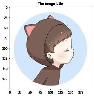
# 3 显示图像
# 3.1 直接显示
# im.show()
# 在 notebook 或者 shell 环境直接 im 即可显示
im

time: 10.7 ms
# 3.2 结合 Plt 显示
plt
.
figure
(
num
=
1
,
figsize
=
(
8
,
5
)
,
)
plt
.
title
(
'The image title'
)
# plt.axis('off') # 不显示坐标轴
plt
.
imshow
(
im
)
plt
.
show
(
)
time: 202 ms
图像处理
图像处理这一块很重要,是以后做图像分类、图像识别等比较重要的图像预处理环节
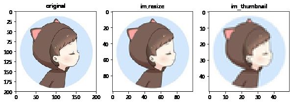
1 图像大小
1-1 缩放大小
im.resize(size, resample)
im.thumbnail(size,resample)(创建缩略图)
保留图片的所有部分,只是缩小或者扩大比例而已
resize 方法可以将原始的图像转换大小,size 是转换之后的大小
resample 是重新采样使用的方法,有以下四种方法,默认 Image.NEAREST
Image.BICUBIC,Image.LANCZOS,Image.BILINEAR,Image.NEAREST
NEAREST:最近滤波。从输入图像中选取最近的像素作为输出像素。它忽略了所有其他的像素。
BILINEAR:双线性滤波。在输入图像的2x2矩阵上进行线性插值。注意:PIL的当前版本,做下采样时该滤波器使用了固定输入模板。
BICUBIC:双立方滤波。在输入图像的4x4矩阵上进行立方插值。注意:PIL的当前版本,做下采样时该滤波器使用了固定输入模板。
ANTIALIAS:平滑滤波。这是PIL 1.1.3版本中新的滤波器。对所有可以影响输出像素的输入像素进行高质量的重采样滤波,
以计算输出像素值。在当前的PIL版本中,这个滤波器只用于改变尺寸和缩略图方法。
注意:在当前的PIL版本中,ANTIALIAS滤波器是下采样(例如,将一个大的图像转换为小图)时唯一正确的滤波器。
BILIEAR和BICUBIC滤波器使用固定的输入模板,用于固定比例的几何变换和上采样是最好的。
from
PIL
import
Image
# 设置画布大小
plt
.
figure
(
figsize
=
(
10
,
8
)
)
# original
im
=
Image
.
open
(
path
)
(
'原图像像素大小:'
,
im
.
size
)
plt
.
subplot
(
131
)
;
plt
.
title
(
'original'
)
plt
.
imshow
(
im
)
# resize()——>返回新的 image 对象
im_resize
=
im
.
resize
(
(
100
,
100
)
,
resample
=
Image
.
LANCZOS
)
(
'im_resize 转换后像素大小:'
,
im_resize
.
size
)
plt
.
subplot
(
132
)
;
plt
.
title
(
'im.resize'
)
plt
.
imshow
(
im_resize
)
# thumbnail()——>直接覆盖原始的 im
im_thumbnail
=
im
.
thumbnail
(
(
50
,
50
)
,
resample
=
Image
.
LANCZOS
)
(
im_thumbnail
)
plt
.
subplot
(
133
)
;
plt
.
title
(
'im_thumbnail'
)
plt
.
imshow
(
im
)
# plt.axis('off') # 不显示坐标轴
plt
.
show
(
)
原图像像素大小: (200, 200)
im_resize 转换后像素大小: (100, 100)
None
time: 427 ms
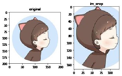
1-2 裁剪大小
im.crop(box)
截取图片,图片部分信息丢失
从当前的图像中返回一个矩形区域的拷贝。
变量box是一个四元组,定义了左、上、右和下的像素坐标。
请注意:box 中距离设置是以 左上角x轴与左上角y轴,即(0, 0)为基准来计算的
from
PIL
import
Image
im
=
Image
.
open
(
path
)
box
=
(
35
,
20
,
160
,
193
)
# 注意理解这里的设置
im_crop
=
im
.
crop
(
box
)
# 显示
plt
.
figure
(
figsize
=
(
7
,
4
)
)
# 设置画布大小
plt
.
subplot
(
121
)
;
plt
.
title
(
'original'
)
plt
.
imshow
(
im
)
plt
.
subplot
(
122
)
;
plt
.
title
(
'im_crop'
)
plt
.
imshow
(
im_crop
)
# plt.axis('off') # 不显示坐标轴
plt
.
show
(
)
time: 308 ms
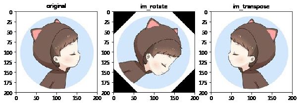
2 图像旋转
transpose()和rotate()没有性能差别
rotate()
rotate(45) 顺时针 45 度
rotate(-45) 逆时针 45 度
transpose(method)(图像翻转或者旋转),method 参数如下
Image.FLIP_LEFT_RIGHT,表示将图像左右翻转
Image.FLIP_TOP_BOTTOM,表示将图像上下翻转
Image.ROTATE_90,表示将图像逆时针旋转90°
Image.ROTATE_180,表示将图像逆时针旋转180°
Image.ROTATE_270,表示将图像逆时针旋转270°
Image.TRANSPOSE,表示将图像进行转置(相当于顺时针旋转90°)
Image.TRANSVERSE,表示将图像进行转置,再水平翻转
%
%
time
from
PIL
import
Image
# 设置画布大小
plt
.
figure
(
figsize
=
(
10
,
5
)
)
im
=
Image
.
open
(
path
)
plt
.
subplot
(
131
)
;
plt
.
title
(
'original'
)
plt
.
imshow
(
im
)
# rotate()
im_rotate
=
im
.
rotate
(
-
45
)
# 顺时针角度表示
plt
.
subplot
(
132
)
;
plt
.
title
(
'im_rotate'
)
plt
.
imshow
(
im_rotate
)
# transpose()
im_transpose
=
im
.
transpose
(
Image
.
FLIP_LEFT_RIGHT
)
# 左右翻转
plt
.
subplot
(
133
)
;
plt
.
title
(
'im_transpose'
)
plt
.
imshow
(
im_transpose
)
# plt.axis('off') # 不显示坐标轴
plt
.
show
(
)
CPU times: user 472 ms, sys: 8 ms, total: 480 ms
Wall time: 476 ms
time: 478 ms
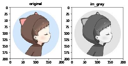
3 图像通道
3-1 颜色通道
im.convert(mode)⇒ image
将当前图像转换为其他模式,并且返回新的图像
mode 的取值可以是如下几种:
1 1位像素,黑和白,存成8位的像素
L8位像素,黑白(灰度图),只有一个颜色通道
P8位像素,使用调色板映射到任何其他模式
RGB3× 8位像素,真彩
RGBA4×8位像素,真彩+透明通道
CMYK4×8位像素,颜色隔离
YCbCr3×8位像素,彩色视频格式
I32位整型像素
F32位浮点型像素
%
%
time
from
PIL
import
Image
# 设置画布大小
plt
.
figure
(
figsize
=
(
10
,
5
)
)
im
=
Image
.
open
(
path
)
(
'原始图像模式:'
,
im
.
mode
)
plt
.
subplot
(
131
)
;
plt
.
title
(
'original'
)
plt
.
imshow
(
im
)
# convert(mode)
im_gray
=
im
.
convert
(
'L'
)
# 加载为灰度图
(
'im_convert 图像模式:'
,
im_gray
.
mode
)
plt
.
subplot
(
132
)
;
plt
.
title
(
'im_gray'
)
plt
.
imshow
(
im_gray
)
# plt.axis('off') # 不显示坐标轴
plt
.
show
(
)
原始图像模式: RGB
im_convert 图像模式: L
CPU times: user 312 ms, sys: 0 ns, total: 312 ms
Wall time: 303 ms
time: 304 ms
如果转换后的图像显示异常
如:AttributeError: ‘numpy.ndarray’ object has no attribute ‘mask’
解决方法 很有可能是版本问题,要更新 matplotlib,如:$ pip install -U matplotlib
3-2 通道分离与合并
split()(颜色通道分离)
r,g,b=img.split() #分离三通道
merge(mode,channels)(颜色通道合并)
pic=Image.merge(‘RGB’,(r,g,b)) #合并三通道
r
,
g
,
b
=
im
.
split
(
)
# 分离三通道
merge
=
Image
.
merge
(
'RGB'
,
(
r
,
g
,
b
)
)
# 合并三通道
merge

time: 11.6 ms
4 图像添加水印
4-1 在图片上面加文字
# 提示:这段代码在科赛里不能运行,
# 可以在自己本地的 notebook 运行
# from PIL import Image, ImageDraw, ImageFont
# im = Image.open(path)
# draw = ImageDraw.Draw(im) # 新建绘图对象
# width, height = im.size # 获取图像的宽和高
# setFont = ImageFont.truetype('C:/windows/fonts/Dengl.ttf', 20) # ImageFont模块
# draw.text(xy=(width - 140, height - 25), # 文字位置
# text=u'吻我别说话hhh', # 文字
# font=setFont, # 字体样式和大小
# fill="blue" # 设置文字颜色
# )
# im
time: 399 µs
4-2 添加文字水印
Signature: Image.alpha_composite(im1, im2)
im1, im2 必须为 RGBA 模式
Docstring:
Alpha composite im2 over im1.
:param im1: The first image. Must have mode RGBA.
:param im2: The second image. Must have mode RGBA, and the same size as
the first image.
# 提示:这段代码在科赛里不能运行,
# 可以在自己本地的 notebook 运行
# from PIL import Image, ImageDraw,ImageFont
# im = Image.open(path).convert('RGBA')
# # 新建图像
# txt = Image.new('RGBA', im.size, (0,0,0,0))
# # 添加文字
# fnt = ImageFont.truetype('C:/windows/fonts/Dengl.ttf', 20)
# d = ImageDraw.Draw(txt)
# d.text(xy=(txt.size[0]-80,txt.size[1]-30),
# text=u"小知同学",
# font=fnt,
# fill='blue'
# )
# # 合并图像
# im = Image.alpha_composite(im, txt)
# im
time: 553 µs
4-3 添加图片水印
这里只是一个小演示,可以准备其他图片水印再添加,效果会更好呢
from
PIL
import
Image
im
=
Image
.
open
(
path
)
watermark
=
Image
.
open
(
path
)
layer
=
Image
.
new
(
'RGBA'
,
im
.
size
,
(
0
,
0
,
0
,
0
)
)
layer
.
paste
(
watermark
,
(
im
.
size
[
0
]
-
150
,
im
.
size
[
1
]
-
60
)
)
im
=
Image
.
composite
(
layer
,
im
,
layer
)
im

time: 15.8 ms
5 图像增强
enhanceImg = ImageEnhance.Contrast(im)
enhanceImg.enhance(2.0).show()
2.0表示增强两倍,1.0表示不增强
from
PIL
import
Image
,
ImageEnhance
import
matplotlib
.
pyplot
as
plt
# 设置画布大小
plt
.
figure
(
figsize
=
(
10
,
8
)
)
# --------------------------------------
# 原始图像
im
=
Image
.
open
(
path
)
plt
.
subplot
(
231
)
;
plt
.
title
(
'original'
)
plt
.
imshow
(
im
)
# ----------图像增强-----------------------
# 增强亮度
# 调整图片的明暗平衡
ie_Brightness
=
ImageEnhance
.
Brightness
(
im
)
plt
.
subplot
(
232
)
;
plt
.
title
(
'ie_Brightness'
)
plt
.
imshow
(
ie_Brightness
.
enhance
(
2.0
)
)
plt
.
axis
(
'off'
)
# 关掉坐标轴
# 图片尖锐化
# 锐化/钝化图片
ie_Sharpness
=
ImageEnhance
.
Sharpness
(
im
)
plt
.
subplot
(
233
)
;
plt
.
title
(
'ie_Sharpness'
)
plt
.
imshow
(
ie_Sharpness
.
enhance
(
2.0
)
)
# 对比度增强
# 调整图片的对比度
ie_Contrast
=
ImageEnhance
.
Contrast
(
im
)
plt
.
subplot
(
234
)
;
plt
.
title
(
'ie_Contrast'
)
plt
.
imshow
(
ie_Contrast
.
enhance
(
2.0
)
)
# 色彩增强
# 图片的色彩平衡,相当于彩色电视机的色彩调整
ie_Color
=
ImageEnhance
.
Color
(
im
)
plt
.
subplot
(
235
)
;
plt
.
title
(
'ie_Color'
)
plt
.
imshow
(
ie_Color
.
enhance
(
2.0
)
)
plt
.
axis
(
'off'
)
# 关掉坐标轴
plt
.
show
(
)

time: 584 ms
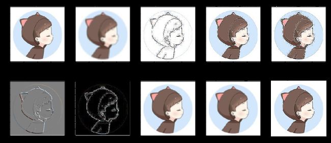
6 图像滤镜
ImageFilter是PIL的滤镜模块,通过这些预定义的滤镜,
可以方便的对图片进行一些过滤操作,从而去掉图片中的噪音(部分的消除),
这样可以降低将来处理的复杂度(如模式识别等)。
滤镜名称 含义
ImageFilter.BLUR 模糊滤镜
ImageFilter.CONTOUR 轮廓
ImageFilter.EDGE_ENHANCE 边界加强
ImageFilter.EDGE_ENHANCE_MORE 边界加强(阀值更大)
ImageFilter.EMBOSS 浮雕滤镜
ImageFilter.FIND_EDGES 边界滤镜
ImageFilter.SMOOTH 平滑滤镜
ImageFilter.SMOOTH_MORE 平滑滤镜(阀值更大)
ImageFilter.SHARPEN 锐化滤镜
# 实际上这个可以使用一个循环来批量处理的
# 读者朋友可以自己试一试
import
matplotlib
.
pyplot
as
plt
from
PIL
import
Image
from
PIL
import
ImageFilter
im
=
Image
.
open
(
path
)
# 设置画布大小
plt
.
figure
(
figsize
=
(
18
,
8
)
)
plt
.
subplot
(
251
)
;
plt
.
title
(
'original'
)
;
plt
.
imshow
(
im
)
im1
=
im
.
filter
(
ImageFilter
.
BLUR
)
# 均值/模糊滤波
plt
.
subplot
(
252
)
;
plt
.
title
(
'ImageFilter.BLUR'
)
;
plt
.
imshow
(
im1
)
im2
=
im
.
filter
(
ImageFilter
.
CONTOUR
)
# 寻找轮廓
plt
.
subplot
(
253
)
;
plt
.
title
(
'ImageFilter.CONTOUR'
)
;
plt
.
imshow
(
im2
)
im3
=
im
.
filter
(
ImageFilter
.
EDGE_ENHANCE
)
# 边界加强
plt
.
subplot
(
254
)
;
plt
.
title
(
'ImageFilter.EDGE_ENHANCE'
)
;
plt
.
imshow
(
im3
)
im4
=
im
.
filter
(
ImageFilter
.
EDGE_ENHANCE_MORE
)
# 边界加强(阀值更大)
plt
.
subplot
(
255
)
;
plt
.
title
(
'ImageFilter.EDGE_ENHANCE_MORE'
)
;
plt
.
imshow
(
im4
)
im5
=
im
.
filter
(
ImageFilter
.
EMBOSS
)
# 浮雕滤镜
plt
.
subplot
(
256
)
;
plt
.
title
(
'ImageFilter.EMBOSS'
)
;
plt
.
imshow
(
im5
)
im6
=
im
.
filter
(
ImageFilter
.
FIND_EDGES
)
# 边界滤镜
plt
.
subplot
(
257
)
;
plt
.
title
(
'ImageFilter.FIND_EDGES'
)
;
plt
.
imshow
(
im6
)
im7
=
im
.
filter
(
ImageFilter
.
SMOOTH
)
# 平滑滤镜
plt
.
subplot
(
258
)
;
plt
.
title
(
'ImageFilter.SMOOTH'
)
;
plt
.
imshow
(
im7
)
im8
=
im
.
filter
(
ImageFilter
.
SMOOTH_MORE
)
# 平滑滤镜(阈值更大)
plt
.
subplot
(
259
)
;
plt
.
title
(
'ImageFilter.SMOOTH_MORE'
)
;
plt
.
imshow
(
im8
)
im9
=
im
.
filter
(
ImageFilter
.
SHARPEN
)
# 锐化滤镜
plt
.
subplot
(
2
,
5
,
10
)
;
plt
.
title
(
'ImageFilter.SHARPEN'
)
;
plt
.
imshow
(
im9
)
plt
.
axis
(
'off'
)
# 关掉坐标轴
plt
.
show
(
)
time: 1.39 s
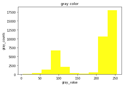
7 图像直方图
7-1 灰度图直方图
多维变换:a.reshape(2,3)
展平为一维:a.ravel()/a.flatten()
import
numpy
as
np
from
PIL
import
Image
import
matplotlib
.
pyplot
as
plt
im
=
Image
.
open
(
path
)
.
convert
(
'L'
)
# 加载图像为灰度
(
'>>>像素大小:'
,
im
.
size
)
im_to_array
=
np
.
array
(
im
)
# 将图像转换成数组
x_value
=
im_to_array
.
flatten
(
)
# 将数组展平为一维数组
result
=
plt
.
hist
(
x
=
x_value
,
# x 轴一维数据
bins
=
None
,
# 柱子的大小,默认为 10(即 None)
color
=
'yellow'
,
# 柱子的颜色
normed
=
0
,
# 是否归一化处理,默认为 0,非 0 就进行归一化处理
alpha
=
0.9
# 柱形图透明度,取值区间 [0, 1]——>[暗,亮]
)
(
'\n>>> X 轴元素对应着出现的次数 n:\n'
,
result
[
0
]
)
(
'\n>>> X 轴元素值 bins:\n'
,
result
[
1
]
)
plt
.
title
(
'gray color'
)
plt
.
xlabel
(
'gray_value'
)
plt
.
ylabel
(
'gray_counts'
)
plt
.
show
(
)
>>>像素大小: (200, 200)
>>> X 轴元素对应着出现的次数 n:
[ 31. 349. 1248. 6690. 2089. 366. 179. 465. 10567. 18016.]
>>> X 轴元素值 bins:
[ 4. 29.1 54.2 79.3 104.4 129.5 154.6 179.7 204.8 229.9 255. ]
time: 186 ms
7-2 彩色图直方图
灰度直方图和彩色直方图差不多,只不过灰度图只有一个颜色通道,而彩色图有多个通道,如 RGB等
from
PIL
import
Image
import
numpy
as
np
import
matplotlib
.
pyplot
as
plt
im
=
Image
.
open
(
path
)
r
,
g
,
b
=
im
.
split
(
)
# 分割颜色通道
r_value
=
np
.
array
(
r
)
.
flatten
(
)
# 将图片转换成数组并展平为一维数组
plt
.
hist
(
x
=
r_value
,
bins
=
30
,
normed
=
0
,
facecolor
=
'r'
,
edgecolor
=
'r'
)
g_value
=
np
.
array
(
g
)
.
flatten
(
)
plt
.
hist
(
x
=
g_value
,
bins
=
30
,
normed
=
0
,
facecolor
=
'g'
,
edgecolor
=
'g'
)
b_value
=
np
.
array
(
b
)
.
flatten
(
)
plt
.
hist
(
x
=
b_value
,
bins
=
30
,
normed
=
0
,
facecolor
=
'b'
,
edgecolor
=
'b'
)
plt
.
title
(
'RGB color'
)
plt
.
xlabel
(
'R_G_B_value'
)
plt
.
ylabel
(
'R_G_B_counts'
)
plt
.
show
(
)

time: 332 ms
8 图像通道运算
暂时不写出来,有空就更新…
图像向量化
将图像向量化之后才能进行相关的算法进行图片分类、模式识别等
1 图像转换为数组
import
numpy
as
np
from
PIL
import
Image
im
=
Image
.
open
(
path
)
im

time: 12.8 ms
im_array
=
np
.
array
(
im
)
(
'>>>图像大小:'
,
im
.
size
)
(
'\n>>>图像通道模式:%s'
%
im
.
mode
)
(
'\n'
,
'---'
*
10
,
'\n>>>图像信息:'
,
im_array
.
shape
)
(
'\n>>>图像宽度:%d \n>>>图像高度:%d \n>>>图像通道数:%d'
%
(
im_array
.
shape
[
0
]
,
im_array
.
shape
[
1
]
,
im_array
.
shape
[
2
]
)
)
(
im_array
[
:
2
]
.
shape
)
im_array
[
:
2
]
>>>图像大小: (200, 200)
>>>图像通道模式:RGB
------------------------------
>>>图像信息: (200, 200, 3)
>>>图像宽度:200
>>>图像高度:200
>>>图像通道数:3
(2, 200, 3)
array([[[255, 255, 255],
[255, 255, 255],
[255, 255, 255],
...,
[255, 255, 255],
[255, 255, 255],
[255, 255, 255]],
[[255, 255, 255],
[255, 255, 255],
[255, 255, 255],
...,
[255, 255, 255],
[255, 255, 255],
[255, 255, 255]]], dtype=uint8)
time: 5.28 ms
2 数组转换成图像
from
PIL
import
Image
im
=
Image
.
open
(
path
)
# 原始图像
im_array
=
np
.
array
(
im
)
# 图像转换成数组
array_im
=
Image
.
fromarray
(
im_array
)
# 数组转换成图像
array_im

time: 13.1 ms
3 图像处理成三维数组
适用于深度学习 CNN 等训练
import
numpy
as
np
from
PIL
import
Image
# resize 统一图像像素
im1
=
np
.
array
(
Image
.
open
(
path
)
.
convert
(
'L'
)
.
resize
(
(
28
,
28
)
)
)
im2
=
np
.
array
(
Image
.
open
(
path
)
.
convert
(
'L'
)
.
resize
(
(
28
,
28
)
)
)
(
im1
.
shape
)
(
im2
.
shape
)
# im1
(28, 28)
(28, 28)
time: 4.89 ms
# 灰色图只有一个通道
im11
=
im1
.
reshape
(
1
,
28
,
28
)
im22
=
im2
.
reshape
(
1
,
28
,
28
)
(
im11
.
shape
)
(
im22
.
shape
)
# im11
(1, 28, 28)
(1, 28, 28)
time: 852 µs
im3
=
np
.
vstack
(
(
im11
,
im22
)
)
# 以行的维度添加
(
im3
.
shape
)
# 设置图形信息
sample_counts
,
channels
,
width
,
height
=
im3
.
shape
[
0
]
,
1
,
im3
.
shape
[
1
]
,
im3
.
shape
[
2
]
im33
=
im3
.
reshape
(
sample_counts
,
# 样本数量
channels
,
# 频道数
height
,
# 一个样本中的行数量
width
# 一个样本中的列数量
)
(
im33
.
shape
)
# 将像素值缩放到 [0 1] 区间
im33
=
im33
/
255
im33
(2, 28, 28)
(2, 1, 28, 28)
array([[[[1., 1., 1., ..., 1., 1., 1.],
[1., 1., 1., ..., 1., 1., 1.],
[1., 1., 1., ..., 1., 1., 1.],
...,
[1., 1., 1., ..., 1., 1., 1.],
[1., 1., 1., ..., 1., 1., 1.],
[1., 1., 1., ..., 1., 1., 1.]]],
[[[1., 1., 1., ..., 1., 1., 1.],
[1., 1., 1., ..., 1., 1., 1.],
[1., 1., 1., ..., 1., 1., 1.],
...,
[1., 1., 1., ..., 1., 1., 1.],
[1., 1., 1., ..., 1., 1., 1.],
[1., 1., 1., ..., 1., 1., 1.]]]])
time: 5.25 ms
4 图像处理成二维数组
适用于机器学习算法,如 sklearn 系列
import
numpy
as
np
from
PIL
import
Image
# 灰度处理后,resize 统一图像像素,并且展平为一维
im1
=
np
.
array
(
Image
.
open
(
path
)
.
convert
(
'L'
)
.
resize
(
(
28
,
28
)
)
)
.
ravel
(
)
im2
=
np
.
array
(
Image
.
open
(
path
)
.
convert
(
'L'
)
.
resize
(
(
28
,
28
)
)
)
.
ravel
(
)
im3
=
np
.
array
(
Image
.
open
(
path
)
.
convert
(
'L'
)
.
resize
(
(
28
,
28
)
)
)
.
ravel
(
)
(
im1
.
shape
)
(
im2
.
shape
)
(
im3
.
shape
)
# im1
(784,)
(784,)
(784,)
time: 6.72 ms
im4
=
np
.
vstack
(
(
im1
,
im2
,
im3
)
)
# 以行的维度添加
(
im4
.
shape
)
# 将像素值缩放到 [0 1] 区间
im4
=
im4
/
255
im4
(3, 784)
array([[1., 1., 1., ..., 1., 1., 1.],
[1., 1., 1., ..., 1., 1., 1.],
[1., 1., 1., ..., 1., 1., 1.]])
time: 3.75 ms
参考文献
https://www.jianshu.com/p/e8d058767dfa
https://blog.csdn.net/zhangziju/article/details/79123275
https://www.cnblogs.com/chimeiwangliang/p/7130434.html
微信公众号:邯郸路220号子彬院 获取更多