一文带你了解python opencv中霍夫变换(Hough transform)的常用操作

---

前言

霍夫变换是一种特征检测(feature extraction)，被广泛应用在图像分析（image analysis）、计算机视觉(computer vision)以及数位影像处理(digital image processing)。霍夫变换是用来辨别找出物件中的特征，例如：线条。他的算法流程大致如下，给定一个物件、要辨别的形状的种类，算法会在参数空间(parameter space)中执行投票来决定物体的形状，而这是由累加空间(accumulator space)里的局部最大值(local maximum)来决定。

---

霍夫直线变换

cv2.HoughLines

lines = cv2.HoughLines(edges,1,np.pi/180,200)

返回一组(rho, theta)列表。rho以像素为单位测量，并且theta以弧度为单位。

第一个参数，输入图像应该是一个二值图像，所以在应用霍夫变换之前应用阈值或使用精明的边缘检测（Canny）。

第二个和第三个参数分别是rho 和theta的精度。

第四个参数是阈值，这意味着它应该被视为一条线的最低投票数。投票数取决于线上的点数。所以它可能代表了应该检测的最小线长。

代码示例

import cv2
import numpy as np
 
img = cv2.imread('../data/sudoku.png')
gray = cv2.cvtColor(img,cv2.COLOR_BGR2GRAY)
edges = cv2.Canny(gray,50,150,apertureSize = 3)
 
lines = cv2.HoughLines(edges,1,np.pi/180,200)
for line in lines:
    rho,theta = line[0]
    a = np.cos(theta)
    b = np.sin(theta)
    x0 = a*rho
    y0 = b*rho
    x1 = int(x0 + 1000*(-b))
    y1 = int(y0 + 1000*(a))
    x2 = int(x0 - 1000*(-b))
    y2 = int(y0 - 1000*(a))
 
    cv2.line(img,(x1,y1),(x2,y2),(0,0,255),2)
 
cv2.imwrite('houghlines3.jpg',img)

cv2.HoughLinesP

lines = cv2.HoughLinesP(edges, rho, theta, threshold, min_line_length, max_line_gap)

HoughLinesP(image, rho, theta, threshold, lines=…, minLineLength=…, maxLineGap=…)

rho参数表示参数极径 r 以像素值为单位的分辨率，这里一般使用 1 像素。

theta参数表示参数极角 \theta 以弧度为单位的分辨率，这里使用 1度。

threshold参数表示检测一条直线所需最少的曲线交点。

lines参数表示储存着检测到的直线的参数对 (x_{start}, y_{start}, x_{end}, y_{end}) 的容器，也就是线段两个端点的坐标。

minLineLength参数表示能组成一条直线的最少点的数量，点数量不足的直线将被抛弃。

maxLineGap参数表示能被认为在一条直线上的亮点的最大距离。

代码示例

rho = 1
theta = np.pi/180
threshold = 30
min_line_length = 50
max_line_gap = 20

line_image = np.copy(image) #creating an image copy to draw lines on

# Run Hough on the edge-detected image
lines = cv2.HoughLinesP(edges, rho, theta, threshold, np.array([]), min_line_length, max_line_gap)

# Iterate over the output "lines" and draw lines on the image copy
for line in lines:
    for x1,y1,x2,y2 in line:
        cv2.line(line_image,(x1,y1),(x2,y2),(255,0,0),5)

plt.figure(dpi=200, figsize=(3, 3))
plt.tick_params(labelsize=5)
plt.imshow(line_image)

skimage.transform.hough_line

h, angles, d = st.hough_line(img_edges)

h: 霍夫变换累积器

angles: 点与x轴的夹角集合，一般为0-179度

distance: 点到原点的距离

代码示例

import skimage.transform as st

h, angles, d = st.hough_line(img_edges)

print("hough space type:",type(h)," data type:",h.dtype," shape: ",h.shape," dimension: ",h.ndim," max:",np.max(h)," min:",np.min(h))
print("angles space type:",type(angles)," data type:",angles.dtype," shape: ",angles.shape," dimension: ",angles.ndim)
print("dist space type:",type(d)," data type:",d.dtype," shape: ",d.shape," dimension: ",d.ndim," max:",np.max(d)," min:",np.min(d))

        
import math 
hough_d = math.sqrt(wide**2 + height**2)
print("hough_d:",hough_d)

angle_step = 0.5 * np.rad2deg(np.diff(angles).mean())
d_step = 0.5 * np.diff(d).mean()
# bounds = (np.rad2deg(angles[0]) - angle_step,
#           np.rad2deg(angles[-1]) + angle_step,
#           d[-1] + d_step, d[0] - d_step)
bounds = (np.rad2deg(angles[0]) + angle_step,
          np.rad2deg(angles[-1]) - angle_step,
          d[-1] - d_step, d[0] + d_step)
print("max angle",np.rad2deg(np.max(angles)),"min angle:",np.rad2deg(np.min(angles)))
print("max d",np.max(d),d[0],"min d",np.min(d),d[-1])

plt.imshow(np.log(1+h),extent=bounds,cmap='gray')
# extent参数 x轴和y轴的极值，取值为一个长度为4的元组或列表，其中，前两个数值对应x轴的最小值和最大值，后两个参数对应y轴的最小值和最大值

霍夫直线检测的一个具体应用————地图上的道路检测

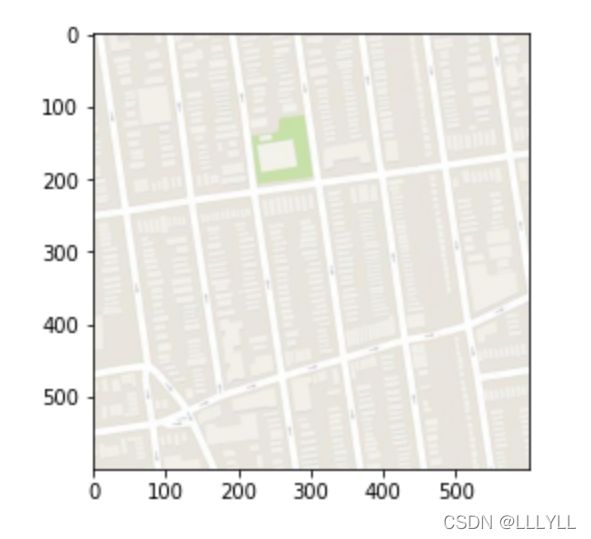
导入资源并显示图像

import numpy as np
import matplotlib.pyplot as plt
import cv2

%matplotlib inline

# Read in the image
image = cv2.imread('map.jpg')

# Change color to RGB (from BGR)
image = cv2.cvtColor(image, cv2.COLOR_BGR2RGB)

plt.imshow(image)

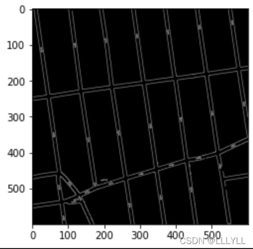
执行边缘检测

# Convert image to grayscale
gray = cv2.cvtColor(image, cv2.COLOR_RGB2GRAY)

# Define our parameters for Canny
low_threshold = 100
high_threshold = 200
edges = cv2.Canny(gray, low_threshold, high_threshold)

plt.imshow(edges, cmap='gray')

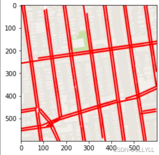
使用Hough变换查找直线

# Define the Hough transform parameters
# Make a blank the same size as our image to draw on
rho = 1
theta = np.pi/180
threshold = 30
min_line_length = 50
max_line_gap = 20

line_image = np.copy(image) #creating an image copy to draw lines on

# Run Hough on the edge-detected image
lines = cv2.HoughLinesP(edges, rho, theta, threshold, np.array([]), min_line_length, max_line_gap)

# Iterate over the output "lines" and draw lines on the image copy
for line in lines:
    for x1,y1,x2,y2 in line:
        cv2.line(line_image,(x1,y1),(x2,y2),(255,0,0),5)
        
plt.imshow(line_image)

lines

Output exceeds the size limit. Open the full output data in a text editor
array([[[ 77, 234, 599, 160]],

       [[400, 183, 459, 599]],

       [[312, 185, 363, 542]],

       [[  9,  30,  69, 453]],

       [[ 76, 244, 599, 170]],

       [[276,   0, 331, 388]],

       [[492, 274, 543, 599]],

       [[110,  78, 153, 384]],

       [[112,  19, 136, 196]],

       [[391, 187, 449, 596]],

       [[501, 269, 552, 597]],

       [[146, 513, 414, 431]],

       [[196,   0, 211, 102]],
...
       [[482, 132, 492, 207]],

       [[486, 229, 501, 329]],

       [[147, 337, 156, 404]]], dtype=int32)

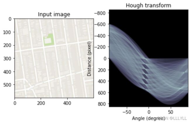
在霍夫空间中展示

import numpy as np
import matplotlib.pyplot as plt

from skimage.transform import hough_line
from skimage.draw import line


out, angles, d = hough_line(edges)


plt.figure(figsize=(20, 10))
fix, axes = plt.subplots(1, 2, figsize=(7, 4))

axes[0].imshow(image, cmap=plt.cm.gray)
axes[0].set_title('Input image')

angle_step = 0.5 * np.rad2deg(np.diff(angles).mean())
d_step = 0.5 * np.diff(d).mean()
bounds = (np.rad2deg(angles[0]) - angle_step,
          np.rad2deg(angles[-1]) + angle_step,
          d[-1] + d_step, d[0] - d_step)

print(np.max(angles),angles[0],np.min(angles),angles[-1])
print(np.max(d),d[0],np.min(d),d[-1])

#axes[1].imshow(out, cmap=plt.cm.bone, extent=bounds)
hough_img = np.log(1+out)
hough_img = cv2.resize(hough_img, dsize=(1699, 1800), fx=5, fy=1)
axes[1].imshow(hough_img, cmap=plt.cm.bone, extent=bounds, aspect='auto')

axes[1].set_title('Hough transform')
axes[1].set_xlabel('Angle (degree)')
axes[1].set_ylabel('Distance (pixel)')

plt.show()

1.5533430342749535 -1.5707963267948966 -1.5707963267948966 1.5533430342749535
849.0 -849.0 -849.0 849.0

霍夫圆变换

cv2.HoughCircles

circles = cv2.HoughCircles(image, method, dp, minDist, circles=None, param1=None, param2=None, minRadius=None, maxRadius=None)

其中：

image:8位，单通道图像。如果使用彩色图像，需要先转换为灰度图像。

method：定义检测图像中圆的方法。目前唯一实现的方法是cv2.HOUGH_GRADIENT。

dp：累加器分辨率与图像分辨率的反比。dp获取越大，累加器数组越小。

minDist：检测到的圆的中心，（x,y）坐标之间的最小距离。如果minDist太小，则可能导致检测到多个相邻的圆。如果minDist太大，则可能导致很多圆检测不到。

param1：用于处理边缘检测的梯度值方法。

param2：cv2.HOUGH_GRADIENT方法的累加器阈值。阈值越小，检测到的圈子越多。

minRadius：半径的最小大小（以像素为单位）。

maxRadius：半径的最大大小（以像素为单位）。

代码示例

circles_im=np.copy(img_copy)
circles=cv2.HoughCircles(gray_blur,cv2.HOUGH_GRADIENT,1,
                         minDist=80,
                         param1=70,
                         param2=20,
                         minRadius=100,
                         maxRadius=150)

circles=np.around(circles).astype('int')
# print(circles)
for i in circles[0]:
    # print(i)
    cv2.circle(circles_im,(i[0],i[1]),i[2],(255,0,0),5)
    cv2.circle(circles_im,(i[0],i[1]),2,(0,255,0),10)
    
plt.imshow(circles_im)

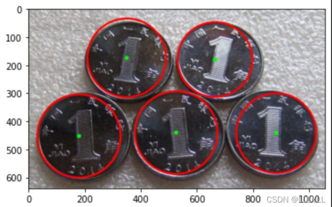
霍夫圆变换的一个具体应用——硬币检测

import related libraries

import cv2
import numpy as np
import matplotlib.pyplot as plt

%matplotlib inline

load image

img = cv2.imread('coins.png')
img_copy=np.copy(img)
img_copy=cv2.cvtColor(img_copy,cv2.COLOR_BGR2RGB)
img_gray=cv2.cvtColor(img_copy,cv2.COLOR_RGB2GRAY)


gray_blur=cv2.GaussianBlur(img_gray,(21,21),cv2.BORDER_DEFAULT)

plt.imshow(img_copy,cmap='gray')
print(gray_blur.shape)

(639, 1056)

HoughCircles function

The HoughCircles function will receive the following variables as its parameters:

• An image, detection method (Hough gradient), resolution factor between detection and image (1),
• minDist-the minimum distance between circle and circle
• param1-the larger value to perform Canny edge detection
• param2-threshold for circle detection, smaller value -> more circles will be detected
• min / max Radius-the minimum and maximum radius of the detected circle

circles_im=np.copy(img_copy)
# TODO
circles=cv2.HoughCircles(gray_blur,cv2.HOUGH_GRADIENT,1,
                         minDist=80,
                         param1=70,
                         param2=20,
                         minRadius=100,
                         maxRadius=150)

circles=np.around(circles).astype('int')
# print(circles)
for i in circles[0]:
    # print(i)
    cv2.circle(circles_im,(i[0],i[1]),i[2],(255,0,0),5)
    cv2.circle(circles_im,(i[0],i[1]),2,(0,255,0),10)
    
plt.imshow(circles_im)

load image

img = cv2.imread('twoCoins.png')
img_copy=np.copy(img)
img_copy=cv2.cvtColor(img_copy,cv2.COLOR_BGR2RGB)
img_gray=cv2.cvtColor(img_copy,cv2.COLOR_RGB2GRAY)


gray_blur=cv2.GaussianBlur(img_gray,(21,21),cv2.BORDER_DEFAULT)

plt.imshow(img_copy,cmap='gray')
print(gray_blur.shape)

(552, 931)

Houghcircle detection

circles_im=np.copy(img_copy)
# TODO
circles=cv2.HoughCircles(gray_blur,cv2.HOUGH_GRADIENT,1,
                         minDist=90,
                         param1=50,
                         param2=20,
                         minRadius=200,
                         maxRadius=220)

circles=np.around(circles).astype('int')
print(circles[0])
for i in circles[0,:]:
    cv2.circle(circles_im,(i[0],i[1]),i[2],(255,0,0),5)
    cv2.circle(circles_im,(i[0],i[1]),2,(0,255,0),20)
    
plt.imshow(circles_im)

[[236 292 200]
[700 292 200]]