深度学习框架TensorFlow学习与应用（二）——非线性回归、MINST数据集分类

非线性回归

import tensorflow as tf
import numpy as np
import matplotlib.pyplot as plt
#使用numpy生成200个随机点
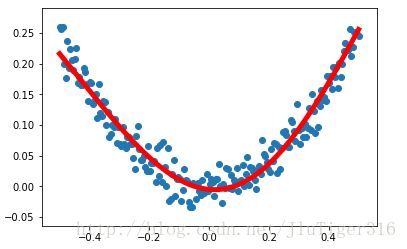
x_data=np.linspace(-0.5,0.5,200)[:,np.newaxis]#-0.5到0.5中均匀分布的200个点，之后增加一个维度
noise=np.random.normal(0,0.02,x_data.shape)#生成干扰，形状和x_data一样
y_data=np.square(x_data)+noise

#定义两个placeholder
x=tf.placeholder(tf.float32,[None,1])
y=tf.placeholder(tf.float32,[None,1])

#定义神经网络中间层,10个神经元
Weight_L1=tf.Variable(tf.random_normal([1,10]))#权值
biases_L1=tf.Variable(tf.zeros([1,1]))#偏置值，10个
Wx_plus_b_L1=tf.matmul(x,Weight_L1)+biases_L1#信号的总和
L1=tf.nn.tanh(Wx_plus_b_L1)#中间层的输出，用双曲正切函数作为激活函数

#定义输出层，1个神经元
Weight_L2=tf.Variable(tf.random_normal([10,1]))
biases_L2=tf.Variable(tf.zeros([1,1]))
Wx_plus_b_L2=tf.matmul(L1,Weight_L2)+biases_L2
prediction=tf.nn.tanh(Wx_plus_b_L2)

#二次代价函数
loss=tf.reduce_mean(tf.square(y-prediction))
#使用梯度下降法训练
train_step=tf.train.GradientDescentOptimizer(0.1).minimize(loss)

with tf.Session() as sess:
    #变量初始化
    sess.run(tf.global_variables_initializer())
    for _ in range(2000):
        sess.run(train_step,feed_dict={x:x_data,y:y_data})

    #获得预测值
    prediction_value=sess.run(prediction,feed_dict={x:x_data})
    #画图
    plt.figure()
    plt.scatter(x_data,y_data)
    plt.plot(x_data,prediction_value,'r-',lw=5)
    plt.show()

得到：

---

MINST数据集分类

1.MNIST数据集

MNIST数据集官网

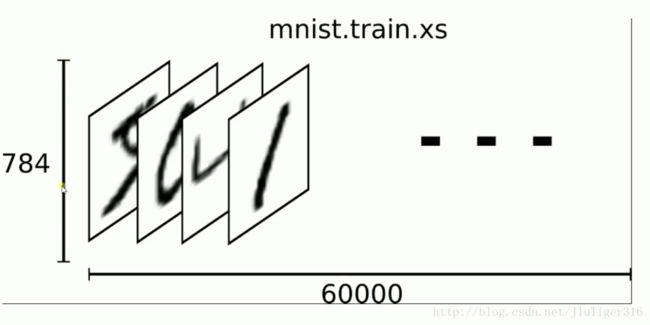
下载下来的数据集被分成两部分：60000行的训练数据集（mnist.train）和10000行的测试数据集（mnise.test）

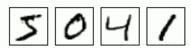
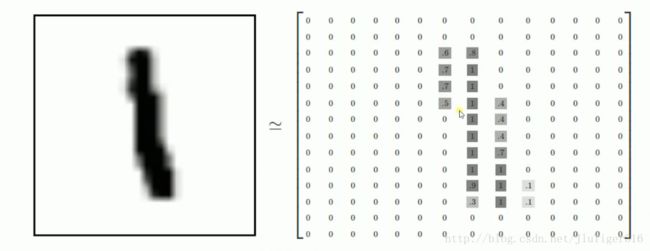
每一张图片包含28*28个像素，我们把这一个数组展开成一个向量，长度是28*28=784。因此在MNIST训练数据集中mnist.train.images是一个形状为[60000，784]的张量，第一个维度数字用来索引图片，第二个维度数字用来索引每张图片的像素点。图片里的某个像素的强度值介于0-1之间。

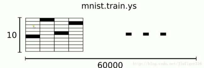
MNIST数据集的标签是介于0-9的数字，我们要把标签转化为“one-hot- vectors”。一个one-hot向量除了某一位数字是1以外，其余维度数字都是0，比如标签0将表示为（[1,0,0,0,0,0,0,0,0,0]）,标签3将表示为（[0,0,0,1,0,0,0,0,0,0]）。
因此，minst.train.labels是一个[60000，10]的数字矩阵。

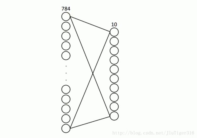
2.神经网络的构建

3.Softmax函数

我们知道MINST的结果是0-9，我们的模型可能推测出一张图片是数字9的概率是80%，是数字8的概率是10%，然后其他数字的概率更小，总体概率加起来等于1。这是一个使用softmax回归模型的经典案例。softmax模型可以用来给不同的对象分配概率。

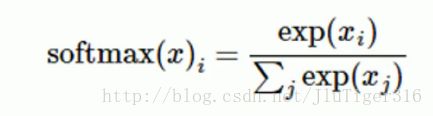
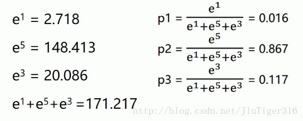
比如输出结果为[1，5，3]

4.MNIST数据集分类简单版本

import tensorflow as tf
from tensorflow.examples.tutorials.mnist import input_data
#载入数据集
mnist=input_data.read_data_sets("D:\BaiDu\MNIST_data",one_hot=True)

#每个批次的大小
batch_size=100
#计算一共有多少个批次
n_batch=mnist.train.num_examples//batch_size

#定义两个placeholder
x=tf.placeholder(tf.float32,[None,784])
y=tf.placeholder(tf.float32,[None,10])#标签

#创建一个简单的神经网络
W=tf.Variable(tf.zeros([784,10]))
b=tf.Variable(tf.zeros([10]))
prediction=tf.nn.softmax(tf.matmul(x,W)+b)

#二次代价函数
loss=tf.reduce_mean(tf.square(y-prediction))
#使用梯度下降法
train_step=tf.train.GradientDescentOptimizer(0.2).minimize(loss)

#初始化变量
init=tf.global_variables_initializer()

#结果存放在一个布尔型列表中
correct_prediction=tf.equal(tf.argmax(y,1),tf.argmax(prediction,1))#比较两个参数大小，相同为true。argmax返回一维张量中最大的值所在的位置
#求准确率
accuracy=tf.reduce_mean(tf.cast(correct_prediction,tf.float32))#将布尔型转化为32位浮点型，再求一个平均值。true变为1.0，false变为0。

with tf.Session() as sess:
    sess.run(init)
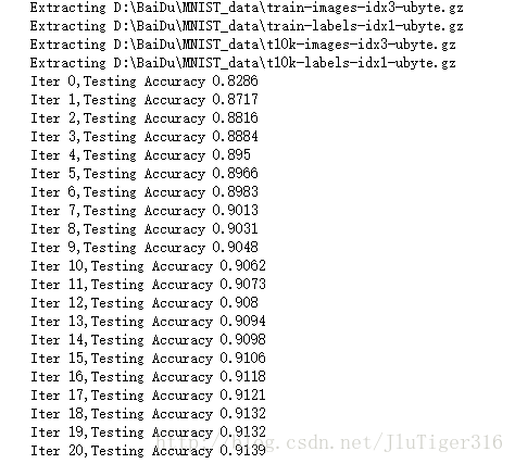
    for epoch in range(21):
        for batch in range(n_batch):
            batch_xs,batch_ys=mnist.train.next_batch(batch_size)
            sess.run(train_step,feed_dict={x:batch_xs,y:batch_ys})

        acc=sess.run(accuracy,feed_dict={x:mnist.test.images,y:mnist.test.labels})
        print("Iter "+str(epoch)+",Testing Accuracy "+str(acc))

运行：