Study Notes- Smoothers and Generalised Additive Models

Preliminaries

Preliminaries
In this practical we will do some model checking and model choice in R.
We need the following packages

• ggplot2 - Package to implement the ggplot language for graphics in R.
• tidyverse - This package is designed to make it easy to install and load multiple ‘tidyverse’ packages in a single step
• MASS - Functions and datasets to support Venables and Ripley, “Modern Applied Statistics with S”(4th edition, 2002).
• caret - For easy machine learning workflow
• splines - Generalized additive (mixed) models, some of their extensions and other generalized ridge regression with multiple smoothing parameter estimation by (Restricted) Marginal Likelihood, Generalized Cross Validation and others

Make sure that these packages are downloaded and installed in R. We use the require() function to load
them into the R library. Note, this does the same as library() in this case.

We will use the Boston data set in the MASS package to predict the median house value (mdev), in Boston
Suburbs, based on the explanatory variable lstat (percentage of lower status of the population).

We want to build some models and then assess how well they do. For this we are going to randomly split
the data into training set (80% for building a predictive model) and evaluation set (20% for evaluating the
model).

As we work through the models we will calculate the usual metrics for model fit, e.g. R2 and RMSE, using
the validation data set, i.e. we will see how well it does at predicting ‘new’ data (out-of-sample validation).

options (warn = -1) # ignore the warnings

require(ggplot2) # input:invalid 可以去掉jupyter 的红色提醒
require(MASS)
require(caret)
require(splines)
require(tidyverse)
require(mgcv)
require(splines2)

Your code contains a unicode char which cannot be displayed in your
current locale and R will silently convert it to an escaped form when the
R kernel executes this code. This can lead to subtle errors if you use
such chars to do comparisons. For more information, please see
https://github.com/IRkernel/repr/wiki/Problems-with-unicode-on-windows

# load the data
data("Boston")
head(Boston)

A data.frame: 6 × 14

	crim	zn	indus	chas	nox	rm	age	dis	rad	tax	ptratio	black	lstat	medv
1	0.00632	18	2.31	0	0.538	6.575	65.2	4.0900	1	296	15.3	396.90	4.98	24.0
2	0.02731	0	7.07	0	0.469	6.421	78.9	4.9671	2	242	17.8	396.90	9.14	21.6
3	0.02729	0	7.07	0	0.469	7.185	61.1	4.9671	2	242	17.8	392.83	4.03	34.7
4	0.03237	0	2.18	0	0.458	6.998	45.8	6.0622	3	222	18.7	394.63	2.94	33.4
5	0.06905	0	2.18	0	0.458	7.147	54.2	6.0622	3	222	18.7	396.90	5.33	36.2
6	0.02985	0	2.18	0	0.458	6.430	58.7	6.0622	3	222	18.7	394.12	5.21	28.7

# Split the data into training and test sets
set.seed(123)
# createDataPartition( )就是数据划分函数，对象是Boston$medv，p=0.8表示训练数据所占的比例为80%，
# list是输出结果的格式，默认list=FALSE。
training.samples<- Boston$medv%>%
    createDataPartition(p= 0.8, list= FALSE)
train.data<- Boston[training.samples, ]
test.data<- Boston[-training.samples, ]

Your code contains a unicode char which cannot be displayed in your
current locale and R will silently convert it to an escaped form when the
R kernel executes this code. This can lead to subtle errors if you use
such chars to do comparisons. For more information, please see
https://github.com/IRkernel/repr/wiki/Problems-with-unicode-on-windows

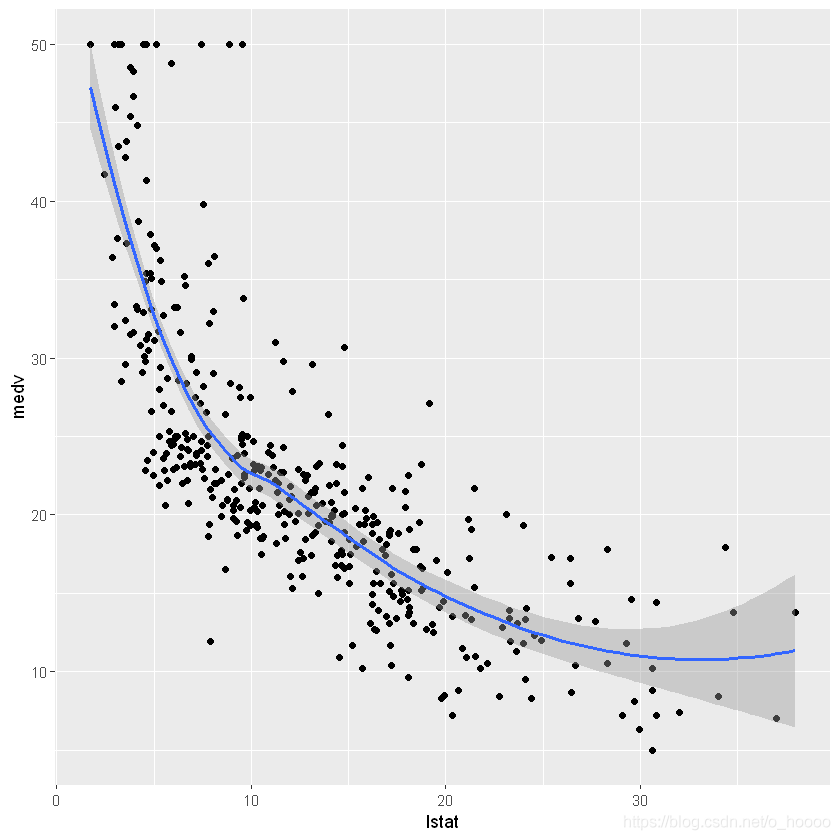
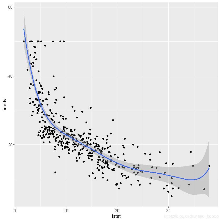
First let’s have a look at the relationship between the two variables

ggplot(train.data, aes(x= lstat, y= medv))+
    geom_point()+
    geom_smooth(method= 'loess', formula= y~ x)

This suggests a non-linear relationship between the two variables.

Linear regression

The standard linear regression model equation can be written as $medv={\beta }_0+{\beta }_1\ast lstat$.

# Fit the model
model1<- lm(medv~ lstat, data= train.data)
summary(model1)

​

Call:
lm(formula = medv ~ lstat, data = train.data)

Residuals:
    Min      1Q  Median      3Q     Max 
-15.218  -4.011  -1.123   2.025  24.459 

Coefficients:
            Estimate Std. Error t value Pr(>|t|)    
(Intercept)  34.6527     0.6230   55.62   <2e-16 ***
lstat        -0.9561     0.0428  -22.34   <2e-16 ***
---
Signif. codes:  0 '***' 0.001 '**' 0.01 '*' 0.05 '.' 0.1 ' ' 1

Residual standard error: 6.144 on 405 degrees of freedom
Multiple R-squared:  0.5521,	Adjusted R-squared:  0.551 
F-statistic: 499.2 on 1 and 405 DF,  p-value: < 2.2e-16

# Make predictions
predictions<- model1 %>%
    predict(test.data)

# Model performance
model1_performance<- data.frame(
    RMSE= RMSE(predictions, test.data$medv), #均方根误差
    # R平方为回归平方和与总离差平方和的比值，表示总离差平方和中可以由回归平方和解释的比例，
    # 这一比例越大越好，模型越精确，回归效果越显著。R平方介于0~1之间，越接近1，回归拟合效果越好
    R2= R2(predictions, test.data$medv)
)

Your code contains a unicode char which cannot be displayed in your
current locale and R will silently convert it to an escaped form when the
R kernel executes this code. This can lead to subtle errors if you use
such chars to do comparisons. For more information, please see
https://github.com/IRkernel/repr/wiki/Problems-with-unicode-on-windows

model1_performance

A data.frame: 1 × 2

RMSE	R2
6.503817	0.513163

This gives a RMSE of 6.503817 and a R2 of 0.513163. The R2 is low, which is not surprising given the relationship is non-linear!

ggplot(data= train.data, aes(x= lstat, y= medv))+
    geom_point()+
    geom_smooth(method= lm, formula= y~ x)

Polynomial regression

A ploynomial regression adds ploynomial or quadratic terms to the regression equations as follows:
$$medv={\beta }_o+bet{a}_1\ast lstat+{\beta }_2\ast lsta{t}^2$$

To create a predictor $x^2$ you can use the function $I()$, e.g $I(x^2)$. This raises x to the power of 2.

model2<- lm(medv~ lstat+ I(lstat^2), data= train.data)model2

​

Call:lm(formula = medv ~ lstat + I(lstat^2), data = train.data)Coefficients:(Intercept)        lstat   I(lstat^2)      42.5736      -2.2673       0.0412  

Or, you can use the poly function:

model2<- lm(medv~ poly(lstat, 2, raw= TRUE), data= train.data)

# Make predictions
predictions2<- model2%>%
    predict(test.data)

# Model perfomance
model2_performance<- data.frame(
    RMSE2= RMSE(predictions2, test.data$medv),
    R22= R2(predictions2, test.data$medv)
)

model2_performance

A data.frame: 1 × 2

RMSE2	R22
5.630727	0.6351934

ggplot(data= train.data, aes(x= lstat, y= medv))+
    geom_point()+
    geom_smooth(method= lm, formula= y~ poly(x, 2, raw= TRUE))

This gives a slightly smaller RMSE (than with the linear model) and an increase in R2 from 0.51 to 0.63.
Not bad, but can we do better?

How about trying a polynomial of order 6?

# Fit the model
model3<- lm(medv~poly(lstat, 6, raw= TRUE), data= train.data)
summary(model3)

​

Call:
lm(formula = medv ~ poly(lstat, 6, raw = TRUE), data = train.data)

Residuals:
     Min       1Q   Median       3Q      Max 
-13.1962  -3.1527  -0.7655   2.0404  26.7661 

Coefficients:
                              Estimate Std. Error t value Pr(>|t|)    
(Intercept)                  7.788e+01  6.844e+00  11.379  < 2e-16 ***
poly(lstat, 6, raw = TRUE)1 -1.767e+01  3.569e+00  -4.952 1.08e-06 ***
poly(lstat, 6, raw = TRUE)2  2.417e+00  6.779e-01   3.566 0.000407 ***
poly(lstat, 6, raw = TRUE)3 -1.761e-01  6.105e-02  -2.885 0.004121 ** 
poly(lstat, 6, raw = TRUE)4  6.845e-03  2.799e-03   2.446 0.014883 *  
poly(lstat, 6, raw = TRUE)5 -1.343e-04  6.290e-05  -2.136 0.033323 *  
poly(lstat, 6, raw = TRUE)6  1.047e-06  5.481e-07   1.910 0.056910 .  
---
Signif. codes:  0 '***' 0.001 '**' 0.01 '*' 0.05 '.' 0.1 ' ' 1

Residual standard error: 5.188 on 400 degrees of freedom
Multiple R-squared:  0.6845,	Adjusted R-squared:  0.6798 
F-statistic: 144.6 on 6 and 400 DF,  p-value: < 2.2e-16

# Make predictions
predictions3<- model3%>%
    predict(test.data)

# Model performance
model3_performance<- data.frame(
    RMSE3= RMSE(predictions3, test.data$medv),
    R23= R2(predictions3, test.data$medv)
)
model3_performance

A data.frame: 1 × 2

RMSE3	R23
5.349512	0.6759031

ggplot(data= train.data, aes(x= lstat, y= medv))+
    geom_point()+
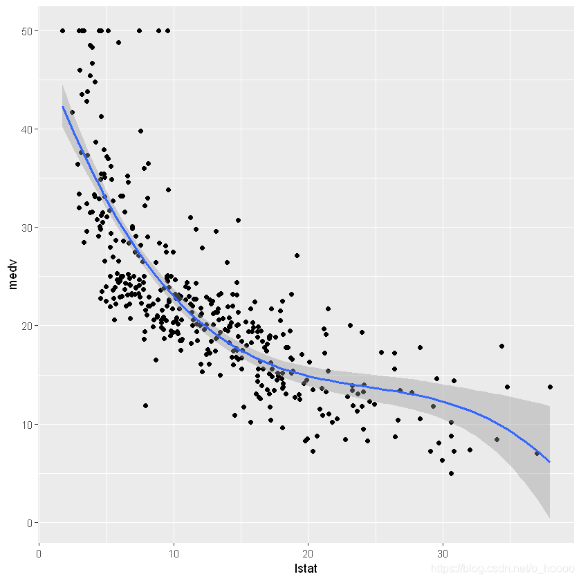
    stat_smooth(method= lm, formula= y~ poly(x, 6, raw= TRUE))

Reduced RMSE and an increase in R2, but counld you interpret the coefficients?

Spline regression

Spline provide a way to smoothly interploate between fixed points, called knots. Polynomial regression is computed between knots. In other words, splines are series of polynomial segments strung together, joining at knots.

The R Package splines2 include the function bSpline for creating a b-spline term in a regression model.

You need to specify two parameters: the degre of the polynomial and the location of the knots.

knots<- quantile(train.data$lstat, p= c(0.25, 0.5, 0.75))

And we will create a model using a cubic spline (each segment has a polynomial regression of degree = 3):

knotes<- quantile(train.data$lstat, p= c(0.25, 0.5, 0.75))
model4<- lm(medv~bSpline(lstat, knots= knots), data= train.data)
# Make predicitions
predictions<- model4%>%
    predict(test.data)
# Model performance
model4_performance<- data.frame(
    RMSE= RMSE(predictions,test.data$medv),
    R2= R2(predictions, test.data$medv)
)
summary(model4)
model4_performance

​

Call:
lm(formula = medv ~ bSpline(lstat, knots = knots), data = train.data)

Residuals:
    Min      1Q  Median      3Q     Max 
-12.952  -3.106  -0.821   2.063  26.861 

Coefficients:
                               Estimate Std. Error t value Pr(>|t|)    
(Intercept)                      52.290      3.344  15.639  < 2e-16 ***
bSpline(lstat, knots = knots)1  -15.740      4.884  -3.223  0.00137 ** 
bSpline(lstat, knots = knots)2  -28.181      3.094  -9.109  < 2e-16 ***
bSpline(lstat, knots = knots)3  -30.083      3.724  -8.077 7.89e-15 ***
bSpline(lstat, knots = knots)4  -41.640      3.713 -11.214  < 2e-16 ***
bSpline(lstat, knots = knots)5  -41.442      5.014  -8.265 2.08e-15 ***
bSpline(lstat, knots = knots)6  -41.308      4.716  -8.760  < 2e-16 ***
---
Signif. codes:  0 '***' 0.001 '**' 0.01 '*' 0.05 '.' 0.1 ' ' 1

Residual standard error: 5.184 on 400 degrees of freedom
Multiple R-squared:  0.685,	Adjusted R-squared:  0.6803 
F-statistic:   145 on 6 and 400 DF,  p-value: < 2.2e-16

A data.frame: 1 × 2

RMSE	R2
5.366847	0.6796817

ggplot(data= train.data, aes(x= lstat, y= medv))+
    geom_point()+
    geom_smooth(method= lm, formula= y~ splines2::bSpline(x, df= 3))

A slight increase in R2, but RMSE has gone up a little.

Generalised additive models

Where you have a non-linear relationship polynomial regression may not be flexible enough to capture the relationship, and spline terms require specifying the knots. Generalised additive models, or GAMs, provide a mechanism to automatically fit a spline regression. i.e you don’t have to choose the knots. This can be done using the mgcv package:

model5<- gam(medv~ s(lstat), data= train.data)
# Make predictions
predictions<- model5%>%
    predict(test.data)
# Model performance
model5_performance<- data.frame(
    RMSE= RMSE(predictions, test.data$medv),
    R2= R2(predictions, test.data$medv)
)
summary(model5)
model5_performance

​

Family: gaussian 
Link function: identity 

Formula:
medv ~ s(lstat)

Parametric coefficients:
            Estimate Std. Error t value Pr(>|t|)    
(Intercept)  22.5106     0.2567   87.69   <2e-16 ***
---
Signif. codes:  0 '***' 0.001 '**' 0.01 '*' 0.05 '.' 0.1 ' ' 1

Approximate significance of smooth terms:
           edf Ref.df     F p-value    
s(lstat) 7.355  8.338 104.1  <2e-16 ***
---
Signif. codes:  0 '***' 0.001 '**' 0.01 '*' 0.05 '.' 0.1 ' ' 1

R-sq.(adj) =  0.681   Deviance explained = 68.7%
GCV = 27.381  Scale est. = 26.819    n = 407

A data.frame: 1 × 2

RMSE	R2
5.318856	0.6760512

ggplot(data= train.data, aes(x= lstat, y= medv))+
    geom_point()+
    geom_smooth(method= gam, formula= y~ s(x))

The term s(lstat) tells the gam() function to fit a smooth function, with the default being to use a ‘penalised’ spline (with the number of knots and their location found using penalty functions).

GAM example - $C{O}_2$ data from Manua Loa

We want to try to identify the intra- (between) and inter- (within) yearly trends.

# Load the data, remember to set the working directory or use Import Dataset
CO2<- read.csv("D:/Code/Datasets/manua_loa_co2.csv", header= TRUE)
head(CO2)

A data.frame: 6 × 4

	year	co2	month	Date
1	1958	315.71	3	1/03/1958
2	1958	317.45	4	1/04/1958
3	1958	317.50	5	1/05/1958
4	1958	317.10	6	1/06/1958
5	1958	315.86	7	1/07/1958
6	1958	314.93	8	1/08/1958

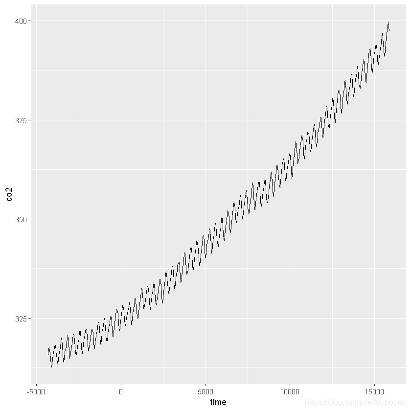
We want to look at inter-annual (within year) trend first. We can convert the data into a continuous time variable (and take a subset for visualisation).

CO2$time<- as.integer(as.Date(CO2$Date, format= "%d/%m/%Y"))
CO2_dat<- CO2
CO2<- CO2[CO2$year %in% (2000: 2010),]
ggplot(CO2_dat, aes(x= time, y= co2))+
    geom_line()

The model being fit here is of the form $y={\beta }_0+f_{trend}(time)+ϵ,ϵN(0,{\sigma }^2)$. We can fit a GAM to these data as follows:

CO2_time<- gam(co2~ s(time), data= CO2, method= "REML")
summary(CO2_time)

​

Family: gaussian 
Link function: identity 

Formula:
co2 ~ s(time)

Parametric coefficients:
            Estimate Std. Error t value Pr(>|t|)    
(Intercept) 379.5817     0.1906    1992   <2e-16 ***
---
Signif. codes:  0 '***' 0.001 '**' 0.01 '*' 0.05 '.' 0.1 ' ' 1

Approximate significance of smooth terms:
        edf Ref.df    F p-value    
s(time)   1  1.001 1104  <2e-16 ***
---
Signif. codes:  0 '***' 0.001 '**' 0.01 '*' 0.05 '.' 0.1 ' ' 1

R-sq.(adj) =  0.894   Deviance explained = 89.5%
-REML = 291.24  Scale est. = 4.7949    n = 132

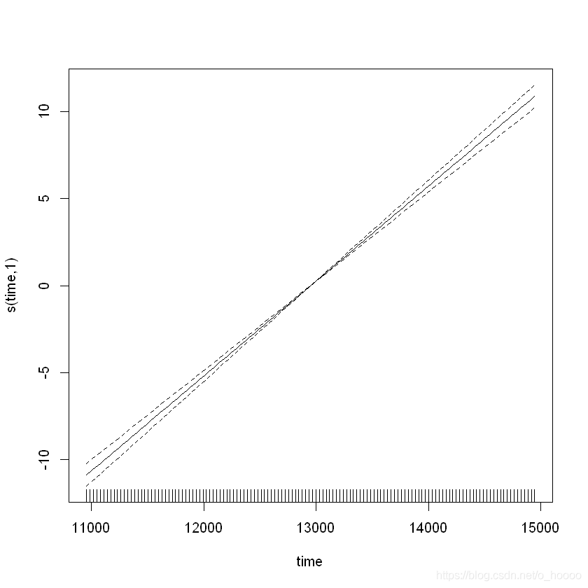
plot(CO2_time)

Note the effective degrees of freedoms (edf) is one, which indicates a linear model. All well and good, until we check how well the model is:

# Split the output into 4 panes
par(mfrow= c(2, 2))
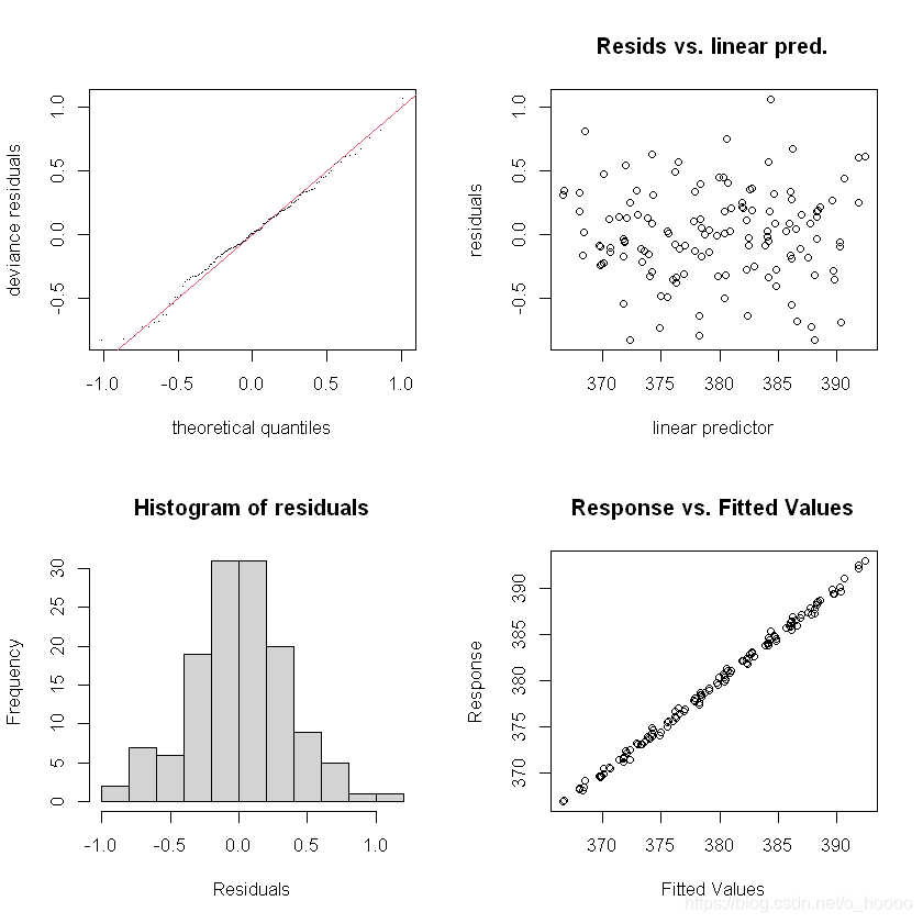
gam.check(CO2_time)

Method: REML   Optimizer: outer newton
full convergence after 8 iterations.
Gradient range [-0.0001447502,6.463421e-05]
(score 291.2359 & scale 4.79491).
Hessian positive definite, eigenvalue range [0.0001447177,64.99994].
Model rank =  10 / 10 

Basis dimension (k) checking results. Low p-value (k-index<1) may
indicate that k is too low, especially if edf is close to k'.

        k' edf k-index p-value    
s(time)  9   1    0.16  <2e-16 ***
---
Signif. codes:  0 '***' 0.001 '**' 0.01 '*' 0.05 '.' 0.1 ' ' 1

The residual have a clear rise-and-fall pattern - clearly there is some within-year patterns. Let’s try again, and introduce something called a cyclical smoother. This will be a model of the form $y={\beta }_0+f_{cyclical}(month)+f_{trend}(time)+ϵ,ϵN(0,\sigma {)}^2$.For the cyclical smoother $f_{cyclical}(month)$ we use the bs=argument to choose the type of smoother, and the k=argument to choose the number of knots (as cubic regression splines have a set number of knots). We use 12 knots, because there are 12 months.

# Fit the model
CO2_season_time<- gam(co2~ s(month, bs= 'cc', k= 12)+ s(time), data= CO2, method= "REML")
# Look at the smoothed terms
par(mfrow= c(1, 2))
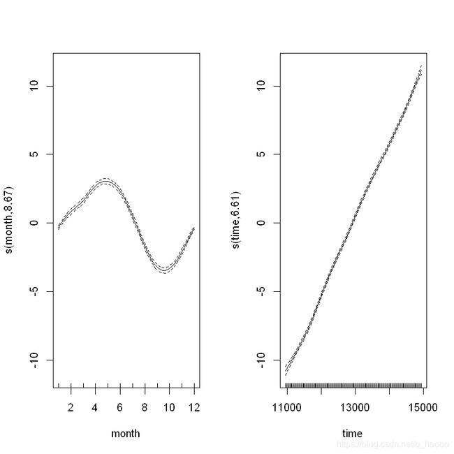
plot(CO2_season_time)

We can see that the cycical smoother is picking up the monthly rise and fall in CO2. Let’s see how the model diagnostics look now:

par(mfrow= c(1, 2))
gam.check(CO2_season_time)

Method: REML   Optimizer: outer newton
full convergence after 6 iterations.
Gradient range [-2.640054e-06,5.25847e-08]
(score 87.72571 & scale 0.1441556).
Hessian positive definite, eigenvalue range [1.026183,65.43149].
Model rank =  20 / 20 

Basis dimension (k) checking results. Low p-value (k-index<1) may
indicate that k is too low, especially if edf is close to k'.

            k'   edf k-index p-value    
s(month) 10.00  8.67    0.72  <2e-16 ***
s(time)   9.00  6.61    0.87   0.045 *  
---
Signif. codes:  0 '***' 0.001 '**' 0.01 '*' 0.05 '.' 0.1 ' ' 1

summary(CO2_season_time)

​

Family: gaussian 
Link function: identity 

Formula:
co2 ~ s(month, bs = "cc", k = 12) + s(time)

Parametric coefficients:
             Estimate Std. Error t value Pr(>|t|)    
(Intercept) 379.58174    0.03305   11486   <2e-16 ***
---
Signif. codes:  0 '***' 0.001 '**' 0.01 '*' 0.05 '.' 0.1 ' ' 1

Approximate significance of smooth terms:
          edf Ref.df      F p-value    
s(month) 8.67  10.00  410.5  <2e-16 ***
s(time)  6.61   7.74 4909.2  <2e-16 ***
---
Signif. codes:  0 '***' 0.001 '**' 0.01 '*' 0.05 '.' 0.1 ' ' 1

R-sq.(adj) =  0.997   Deviance explained = 99.7%
-REML = 87.726  Scale est. = 0.14416   n = 132

Much better indeed - residuals look normally distributed with no obvious pattern time。
What are the R2 and RMSE for this method? Are they better than for the long-term trend model?