bamlss简介
bamlss-A Lego Toolbox for Flexible Bayesian Regression (and Beyond)
一个灵活的贝叶斯回归乐高工具箱
作者: Nikolaus Umlauf, Nadja Klein, Achim Zeileis, Thorsten Simon
原网址
简介:
R包,模块化的计算框架
亮点:
- 与常用的R统计包一样的操作
- GAM-type
- GAMLSS-type
- 模块化的训练过程或者采样过程
尤其是最后一点,bamlss不局限于某一个特定的估计算法,不同的估计算法可以同时使用,并且不需要额外的改变模型的设置。
安装
稳定版本
install.packages("bamlss")
开发版本
install.packages("bamlss", repos = "http://R-Forge.R-project.org")
基本的贝叶斯回归
data("Golf", package = "bamlss")
head(Golf)
##   price age kilometer tia abs sunroof
## 1  7.30  73        10  12 yes     yes
## 2  3.85 115        30  20 yes      no
## 3  2.95 127        43   6  no     yes
## 4  4.80 104        54  25 yes     yes
## 5  6.20  86        57  23  no      no
## 6  5.90  74        57  25 yes      no
建立价格与年龄、公里数等因子之间的关系、
f <- price ~ age + kilometer + tia + abs + sunroof
library("bamlss")

set.seed(111)

b1 <- bamlss(f, family = "gaussian", data = Golf)
MCMC 默认的采样次数为1200, burnin-phase 是200,thinning 是1。
bamlss支持的分布,此外bamlss还支持GAMLSS提供的分布。
summary(b1)
##
## Call:
## bamlss(formula = f, family = "gaussian", data = Golf)
## ---
## Family: gaussian
## Link function: mu = identity, sigma = log
## *---
## Formula mu:
## ---
## price ~ age + kilometer + tia + abs + sunroof
## -
## Parametric coefficients:
##                  Mean      2.5%       50%     97.5% parameters
## (Intercept)  9.333318  8.526293  9.330200 10.173709      9.311
## age         -0.038461 -0.045355 -0.038341 -0.031706     -0.038
## kilometer   -0.009686 -0.012547 -0.009667 -0.007061     -0.010
## tia         -0.005811 -0.022870 -0.005752  0.010105     -0.005
## absyes      -0.240481 -0.492048 -0.237776 -0.003060     -0.238
## sunroofyes  -0.024021 -0.300878 -0.025127  0.238145     -0.010
## -
## Acceptance probability:
##       Mean 2.5% 50% 97.5%
## alpha    1    1   1     1
## ---
## Formula sigma:
## ---
## sigma ~ 1
## -
## Parametric coefficients:
##                Mean    2.5%     50%   97.5% parameters
## (Intercept) -0.2457 -0.3479 -0.2465 -0.1274     -0.271
## -
## Acceptance probability:
##         Mean   2.5%    50% 97.5%
## alpha 0.9703 0.7652 1.0000     1
## ---
## Sampler summary:
## -
## DIC = 408.9675 logLik = -201.0372 pd = 6.8932
## runtime = 1.643
## ---
## Optimizer summary:
## -
## AICc = 409.6319 edf = 7 logLik = -197.4745
## logPost = -252.2614 nobs = 172 runtime = 0.025
这里只展示了对intercepts的曲线,
alpha参数表明很高的接受率,这也是混合好的一个迹象,mixing 可以用图示的方式判断
plot(b1, which = "samples")
tia与sunroof对价格基本没影响,因为估计的参数的置信区间里面包含零,可以使用confint()函数来提取置信区间信息。
confint(b1, prob = c(0.025, 0.975))
##                          2.5%        97.5%
## mu.(Intercept)     8.52629257 10.173709336
## mu.age            -0.04535461 -0.031705531
## mu.kilometer      -0.01254739 -0.007060627
## mu.tia            -0.02286985  0.010105028
## mu.absyes         -0.49204765 -0.003060006
## mu.sunroofyes     -0.30087769  0.238144948
## sigma.(Intercept) -0.34791813 -0.127380063
因为价格不可能是负数,所以使用log对价格进行变化。
set.seed(111)

f <- log(price) ~ age + kilometer + tia + abs + sunroof

b2 <- bamlss(f, family = "gaussian", data = Golf)
比较模型可以使用DIC()
DIC(b1,b2)
##          DIC       pd
## b1 408.96754 6.893153
## b2 -15.19596 6.893153
set.seed(222)

f <- log(price) ~ poly(age, 3) + poly(kilometer, 3) + poly(tia, 3) + abs + sunroof

b3 <- bamlss(f, family = "gaussian", data = Golf)
DIC(b1,b2,b3)
##          DIC        pd
## b1 408.96754  6.893153
## b2 -15.19596  6.893153
## b3 -10.78925 13.186991
结果表示,三次项对模型没有贡献,然后这也可能是由于不显著因子tia的作用。
从图形结果中比较效果可以用使用predict()方法。
与其他包的不同之一就是可以对模型中的单个变量进行预测,数据集中不需要包含所有变量。
例如,对年龄age估计95%的置信区间
nd <- data.frame("age" = seq(min(Golf$age), max(Golf$age), length = 100))

nd$page <- predict(b3, newdata = nd, model = "mu", term = "age",
  FUN = c95, intercept = FALSE)

head(nd)
##        age page.2.5% page.Mean page.97.5%
## 1 65.00000 0.3085312 0.4849915  0.6592331
## 2 65.77778 0.3120472 0.4757206  0.6362999
## 3 66.55556 0.3167776 0.4663256  0.6152946
## 4 67.33333 0.3172396 0.4568109  0.5950657
## 5 68.11111 0.3201536 0.4471811  0.5742218
## 6 68.88889 0.3202023 0.4374406  0.5555146
nd$kilometer <- seq(min(Golf$kilometer), max(Golf$kilometer), length = 100)
nd$tia <- seq(min(Golf$tia), max(Golf$tia), length = 100)
nd$pkilometer <- predict(b3, newdata = nd, model = "mu", term = "kilometer",
  FUN = c95, intercept = FALSE)
nd$ptia <- predict(b3, newdata = nd, model = "mu", term = "tia",
  FUN = c95, intercept = FALSE)
FUN 可以是任何函数, 应用到线性预报因子
par(mfrow = c(1, 3))
ylim <- range(c(nd$page, nd$pkilometer, nd$ptia))
plot2d(page ~ age, data = nd, ylim = ylim)
plot2d(pkilometer ~ kilometer, data = nd, ylim = ylim)
plot2d(ptia ~ tia, data = nd, ylim = ylim)

图中可以清楚的看出因子age与kilometer是负的影响对log的price,然而根据95%的置信区间,tia这个变量是不显著的,因为包含与0水平线。
location- scale模型
这部分例子使用的是摩托车事故数据集
data("mcycle", package = "MASS")
head(mcycle)
##   times accel
## 1   2.4   0.0
## 2   2.6  -1.3
## 3   3.2  -2.7
## 4   3.6   0.0
## 5   4.0  -2.7
## 6   6.2  -2.7
建立高斯均值方差模型
accel ∼ N ( μ = f ( times ) , log ( σ ) = f ( times ) ) \text { accel } \sim \mathcal{N}(\mu=f(\text { times }), \log (\sigma)=f(\text { times })) accel ∼N(μ=f( times ),log(σ)=f( times ))
f <- list(accel ~ s(times, k = 20), sigma ~ s(times, k = 20))
这里s()是mgcv包里面的优化项,这里用list表示公式里面需要估计的参数,te(), ti()也同样支持。
set.seed(123)
b <- bamlss(f, data = mcycle, family = "gaussian")
使用默认的MCMC 采样迭代1200次可以很快获得结果。
首先是使用backfitting 算法获得后验模型估计,之后这些估计值被当做MCMC链的初始值。
返回的模型可以用summary(),plot(),predict()这些通用函数提取信息。
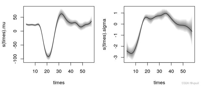
例如,估计的影响对参数mu和sigma可以用下面的命令
plot(b, model = c("mu","sigma"))
模型的总结信息
summary(b)
##
## Call:
## bamlss(formula = f, family = "gaussian", data = mcycle)
## ---
## Family: gaussian
## Link function: mu = identity, sigma = log
## *---
## Formula mu:
## ---
## accel ~ s(times, k = 20)
## -
## Parametric coefficients:
##               Mean   2.5%    50%  97.5% parameters
## (Intercept) -25.13 -29.36 -25.35 -20.34     -25.14
## -
## Acceptance probability:
##       Mean 2.5% 50% 97.5%
## alpha    1    1   1     1
## -
## Smooth terms:
##                     Mean      2.5%       50%     97.5% parameters
## s(times).tau21 425657.47 175634.81 372121.15 914429.32   209325.2
## s(times).alpha      1.00      1.00      1.00      1.00         NA
## s(times).edf       14.24     12.64     14.22     15.97       13.6
## ---
## Formula sigma:
## ---
## sigma ~ s(times, k = 20)
## -
## Parametric coefficients:
##              Mean  2.5%   50% 97.5% parameters
## (Intercept) 2.680 2.549 2.676 2.831      2.581
## -
## Acceptance probability:
##         Mean   2.5%    50% 97.5%
## alpha 0.9664 0.7510 1.0000     1
## -
## Smooth terms:
##                     Mean      2.5%       50%     97.5% parameters
## s(times).tau21 1.458e+02 2.384e+01 1.213e+02 4.604e+02     81.406
## s(times).alpha 5.385e-01 7.903e-04 5.069e-01 1.000e+00         NA
## s(times).edf   9.415e+00 6.491e+00 9.500e+00 1.259e+01      8.675
## ---
## Sampler summary:
## -
## DIC = 1115.068 logLik = -545.2265 pd = 24.6149
## runtime = 4.328
## ---
## Optimizer summary:
## -
## AICc = 1123.881 edf = 24.2718 logLik = -531.975
## logPost = -747.4106 nobs = 133 runtime = 0.463
总结的信息中包括接受率alpha,
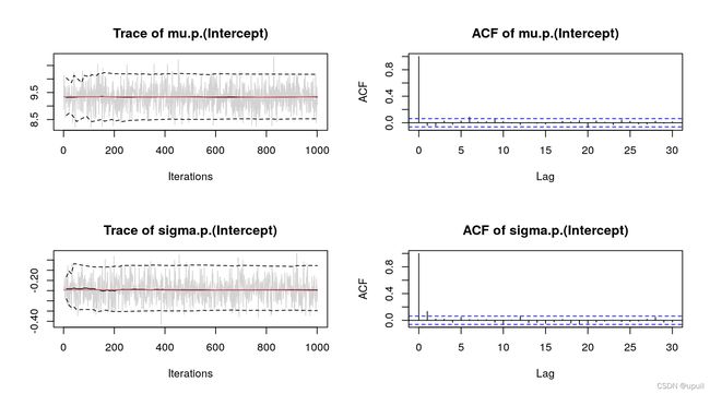
plot(b, which = "samples")
注意,这个命令可以将所有因子的曲线都显示,但是这里只显示截距的曲线。

从迭代曲线中可以看出参数mu并没有辐合
可以调整迭代次数相应的调整thinning参数,
此外,所有参数的最大自相关使用 plot.bamlss 中which="max-acf"
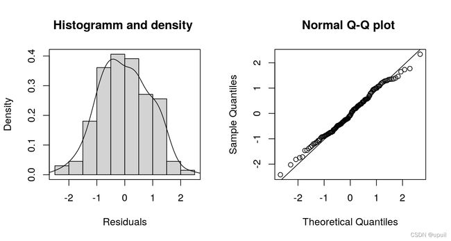
plot(b, which = c("hist-resid", "qq-resid"))
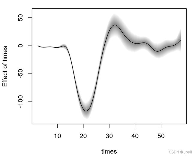
对参数mu后验均值包括95%的置信区间对新数据基于MCMC采样可以这样计算。
nd <- data.frame("times" = seq(2.4, 57.6, length = 100))
nd$ptimes <- predict(b, newdata = nd, model = "mu", FUN = c95)
plot2d(ptimes ~ times, data = nd)
FUN 里面可以是任何函数,例如,可以用identity()函数计算其他分布的统计,画出MCMC采样迭代在times = 10和times = 40时估计的概率密度函数。
## Predict for the two scenarios.
nd <- data.frame("times" = c(10, 40))
ptimes <- predict(b, newdata = nd, FUN = identity, type = "parameter")

## Extract the family object.
fam <- family(b)

## Compute densities.
dens <- list("t10" = NULL, "t40" = NULL)
for(i in 1:ncol(ptimes$mu)) {
  ## Densities for times = 10.
  par <- list(
    "mu" = ptimes$mu[1, i, drop = TRUE],
    "sigma" = ptimes$sigma[1, i, drop = TRUE]
  )
  dens$t10 <- cbind(dens$t10, fam$d(mcycle$accel, par))

  ## Densities for times = 40.
  par <- list(
    "mu" = ptimes$mu[2, i, drop = TRUE],
    "sigma" = ptimes$sigma[2, i, drop = TRUE]
  )
  dens$t40 <- cbind(dens$t40, fam$d(mcycle$accel, par))
}

## Visualize.
par(mar = c(4.1, 4.1, 0.1, 0.1))
col <- rainbow_hcl(2, alpha = 0.01)
plot2d(dens$t10 ~ accel, data = mcycle,
  col.lines = col[1], ylab = "Density")
plot2d(dens$t40 ~ accel, data = mcycle,
  col.lines = col[2], add = TRUE)

参考文献
Dunn, Peter K., and Gordon K. Smyth. 1996. “Randomized Quantile Residuals.” Journal of Computational and Graphical Statistics 5 (3). American Statistical Association, Institute of Mathematical Statistics,; Interface Foundation of America: 236–44.
Fahrmeir, Ludwig, Thomas Kneib, Stefan Lang, and Brian Marx. 2013. Regression – Models, Methods and Applications. Berlin: Springer-Verlag.
Plummer, Martyn, Nicky Best, Kate Cowles, and Karen Vines. 2006. “coda: Convergence Diagnosis and Output Analysis for MCMC.” R News 6 (1): 7–11. https://doi.org/10.18637/jss.v021.i11.
Silverman, B. W. 1985. “Some Aspects of the Spline Smoothing Approach to Non-Parametric Regression Curve Fitting.” Journal of the Royal Statistical Society. Series B (Methodological) 47 (1). [Royal Statistical Society, Wiley]: 1–52.
Umlauf, Nikolaus, Nadja Klein, and Achim Zeileis. 2018. “BAMLSS: Bayesian Additive Models for Location, Scale and Shape (and Beyond).” Journal of Computational and Graphical Statistics 27 (3): 612–27. https://doi.org/10.1080/10618600.2017.1407325.
Umlauf, Nikolaus, Nadja Klein, Achim Zeileis, and Thorsten Simon. 2021a. bamlss: Bayesian Additive Models for Location Scale and Shape (and Beyond). https://CRAN.R-project.org/package=bamlss.
———. 2021b. “bamlss: Bayesian Additive Models for Location Scale and Shape (and Beyond).” Journal of Statistical Software 100 (4): 1–53. https://doi.org/10.18637/jss.v100.i04.
Wood, S. N. 2020. mgcv: GAMs with Gcv/Aic/Reml Smoothness Estimation and Gamms by Pql. https://CRAN.R-project.org/package=mgcv.