2022.12.18 学习周报

---

摘要

This week, I read a paper on recurrent neural networks that explores different ways to extend RNN to deep RNN. Through the understanding and analysis of RNN structure, the paper finds that the network can be deepened from three aspects: input to hidden function, hidden to hidden transformation function and hidden to output function. Based on these observations, several novel deep RNN structures are proposed in this paper, and the results show that the deep RNN is superior to the traditional shallow RNN. In the study of recurrent neural network, I continue to learn the GRU principle, complete the mathematical derivation of GRU formula, and build a simple GRU network model with codes.

本周，我阅读了一篇关于循环神经网络的论文，论文旨在探索将RNN扩展到深度RNN的不同方法。论文通过对RNN结构的理解和分析，发现从三个方面入手可以使网络变得更深， 输入到隐含函数，隐含到隐含转换函数以及隐含到输出函数。基于此类观察结果，论文提出了几种新颖的深度RNN结构，并通过实验验证了深度RNN优于传统的浅层RNN。在循环神经网络的学习中，我继续学习了GRU原理，完成了对GRU公式的数学推导，以及用代码搭建了一个简单的GRU网络模型。

---

文献阅读

1.题目

文献链接：How to Construct Deep Recurrent Neural Networks

2.摘要

In this paper, we explore different ways to extend a recurrent neural network (RNN) to a deep RNN. We start by arguing that the concept of depth in an RNN is not as clear as it is in feedforward neural networks. By carefully analyzing and understanding the architecture of an RNN, however, we find three points of an RNN which may be made deeper; (1) input-to-hidden function, (2) hidden-to-hidden transition and (3) hidden-to-output function. Based on this observation, we propose two novel architectures of a deep RNN which are orthogonal to an earlier attempt of stacking multiple recurrent layers to build a deep RNN (Schmidhuber, 1992; El Hihi and Bengio, 1996). We provide an alternative interpretation of these deep RNNs using a novel framework based on neural operators. The proposed deep RNNs are empirically evaluated on the tasks of polyphonic music prediction and language modeling. The experimental result supports our claim that the proposed deep RNNs benefit from the depth and outperform the conventional, shallow RNNs.

3.介绍

背景：论文中提到RNN和前馈神经网络一样去堆叠网络深度，可以产生具有影响力的模型，但不一样的是RNN的深度是比较模糊的，因为RNN的隐藏层在时间上展开时，可以表示为多个非线性层的组合，因此RNN已经足够深了。

思路：作者研究了将RNN扩展到深层RNN的方法，首先研究了RNN的哪些部分可能被认为是浅层的，然后对每一个浅层部分，提出一种可以替代的更深层的设计，这会导致RNN出现很多更深的变体。

4.RNN

RNN是模拟具有输入xt，输出yt和隐含状态ht的离散时间动态系统，动态系统被定义为：

其中：下标t表示时间，fh表示状态转换函数，fo表示输出函数，每个函数由一组参数（θh和θo）进行优化。

给定一组有N个参数的训练序列，通过最小化代价函数去更新RNN的参数：

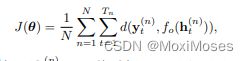
其中d(a, b)是a和b之间的预定义散度测度，例如欧式距离或者交叉熵。

Conventional Recurrent Neural Networks

将转换函数和输出函数定义为：

其中：W，U和V分别为转换矩阵，输入矩阵和输出矩阵，Φh和Φo是逐元素的非线性函数。通常，对于Φh使用饱和非线性函数，例如sigmoid函数或tanh函数。

5.Deep Recurrent Neural Networks

在前馈神经网络中，深度被定义为在输入和输出之间具有的多个非线性层。但不幸的是，由于RNN的时间结构，该定义不适用在RNN中。如下图所示，在时间上展开的RNN都很深，因为在时间k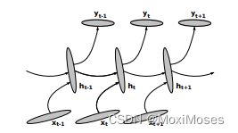
然而，对于RNN在每个时间步上的分析表明，某些转换并不深，而仅仅是线性投影的结果。因此，在没有中间非线性隐含层的情况下，隐含-隐含(ht-1 → ht)，隐含-输出(ht → yt)和输入-隐含(xt → ht)函数都是浅的。

论文中提到可以通过这些转换来思考RNN深度的不同类型，通过在两个连续的隐含状态(ht-1和ht)之间具有一个或多个中间非线性层，可以使隐含-隐含的转换更深。同时，通过在隐含状态ht和输出yt之间插入多个中间非线性层，可以使隐含-输出函数更深。

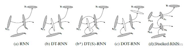
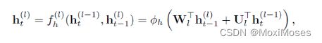
5.1 Deep Transition RNN

从RNN模拟的动态系统的状态转移方程中可以发现，fh的形式没有限制。因此，论文中建议使用多层感知器来代替fh。

其中：Φl表示第l层的单元非线性函数，Wl表示第l层的权重矩阵。

5.2 Deep Output

与上述类似，论文中提出可以使用具有L个中间层的多层感知器来建立下图中的输出函数fo：

其中：Φl表示第l层的单元非线性函数，Vl表示第l层的权重矩阵。

5.3 Stacked RNN

堆叠式RNN具有多个层次的转换函数，其定义为：

其中：ht,l表示在时间t时，第l层的隐含状态。当l = 1时，使用xt代替ht,l来计算状态。

6.实验

论文实验比较了RNN、DT(S)-RNN、DOT(S)-RNN和sRNN 2 layers这4种模型，其中每个模型的大小的选择都给定了范围，以保证实验结果的准确性。

6.1 训练

本实验使用了随机梯度下降法和裁剪梯度的策略，当代价函数停止降低时，训练结束。

在Polyphonic Music Prediction实验中，为了正则化模型，论文在每次计算梯度时，将标准偏差0.075的高斯白噪声添加到每个权重参数中。

在Language Modeling实验中，学习率从初始值开始，每次代价函数没有显著降低时，学习率减半。实验中不使用任何正则化来进行字符级建模，但对于单词级建模，实验会添加权重噪声。

6.2 结果与分析

如下图所示，展示了四种不同模型在同一数据集上的表现结果。

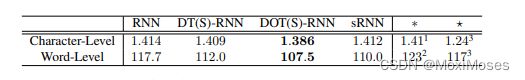
从上图的数据可以表明，深度RNN的表现都优于传统的浅层RNN，但每个深度RNN的适用性取决于其所训练的数据。

7.讨论

论文中提到在实验中遇到了一个实际问题是训练深度RNN的难度。训练传统的RNN是比较容易的，但训练深度RNN是比较困难的，因此论文中提出使用short connection以及常规RNN对它们进行预处理。然而，作者认为随着模型的大小和深度的增加，训练可能会变得更加困难。因此，在未来发现这一困难的根本原因和探索潜在的解决方案将非常重要，论文中提出可以使用advanced regularization methods和advanced optimization algorithms等有效的方法。

深度学习

GRU公式推导

GRU神经网络的整体结构与RNN神经网络的整体结构基本相同，区别是GRU在隐藏层中引入了门控单元。

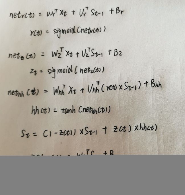
1.GRU前向传播

1）将上一时刻神经单元的输出St-1和当前时刻的输入Xt合并输入到r(t)中去。
2）将上一时刻神经单元的输出St-1和当前时刻的输入Xt合并输入到z(t)中。
3）将上面计算出来的r(t)和St−1进行对位相乘，再将计算结果与Xt进行加法合并。
4）将上面三个步骤计算出来的结果结合起来更新St，最后计算出输出值。

2.GRU反向传播

误差函数选用交叉熵函数，交叉熵函数公式为：

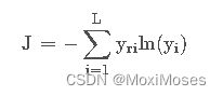
其中：yri表示真实标签值的第i个属性，yi表示预测值的第i个属性。

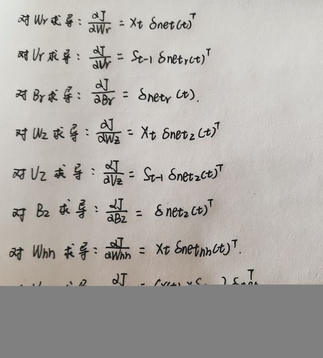
1）偏导计算

2）权重矩阵参数梯度

GRU代码实现

1）GRU代码逐行实现

import torch
from torch import nn
import torch.nn.functional as F


class GRU(nn.Module):
    def __init__(self, indim, hidim, outdim):
        super(GRU, self).__init__()

        # 输入层维度 隐藏层维度 输出层维度
        self.indim = indim
        self.hidim = hidim
        self.outdim = outdim

        # 权重矩阵初始化
        self.w_zh, self.w_zx, self.b_z = self.get_three_parameters()
        self.w_rh, self.w_rx, self.b_r = self.get_three_parameters()
        self.w_hh, self.w_hx, self.b_h = self.get_three_parameters()

        self.Linear = nn.Linear(hidim, outdim)

    def get_three_parameters(self):
        return nn.Parameter(torch.FloatTensor(self.hidim, self.hidim)), \
               nn.Parameter(torch.FloatTensor(self.indim, self.hidim)), \
               nn.Parameter(torch.FloatTensor(self.hidim))

    def forward(self, input, state):
        input = input.type(torch.float32)
        Y = []
        h = state
        for x in input:
            z = F.sigmoid(h @ self.w_zh + x @ self.w_zx + self.b_z)
            r = F.sigmoid(h @ self.w_rh + x @ self.w_rx + self.b_r)
            ht = F.tanh((h * r) @ self.w_hh + x @ self.w_hx + self.b_h)
            h = (1 - z) * h + z * ht
            y = self.Linear(h)
            Y.append(y)
        return torch.cat(Y, dim=0), h

2）GRU API实现

import torch
from torch import nn


class GRU(nn.Module):
    def __init__(self, indim, hidim, outdim):
        super(GRU, self).__init__()
        self.GRU = nn.GRU(indim, hidim)
        self.Linear = nn.Linear(hidim, outdim)

    def forward(self, input, state):
        input = input.type(torch.float32)
        h = state.unsqueeze(0)
        y, state = self.GRU(input, h)
        output = self.Linear(y.reshape(-1, y.shape[-1]))
        return output, state

---

总结

本周，我继续学习了循环神经网络相关内容，完成了对GRU的公式推导和代码实现，认识到GRU比上周学到的LSTM简单，参数量更少，训练速度更快，因此适用于构建较大的网络。而且GRU只有两个门控，从计算角度上来看，它的效率更高，它的可扩展性有利于构建较大的模型，但是LSTM因为有三个门控，更加的强大和灵活，表达能力更强，同时训练速度会比GRU慢一些。