【论文】Legal Judgment Prediction via Topological Learning

• 该论文发表于：EMNLP 2018
  

摘要

1. Legal Judgment Prediction (LJP) ： 基于案件的事实来预测审判结果。
2. 法律审判由多个子任务组成： the decisions of applicable law articles（可用法条）, charges（罪名指控）, fines（罚金）, and the term of penalty（处罚）.
3. 存在问题：现有的工作仅仅关注 judgment Prediction（审判预测）中的特定的子任务，而忽略了子任务之间的拓扑依赖关系。
4. 解决方法：本文将子任务之间的依赖视为有向无环图（DAG），并提出一个拓扑的多任务学习框架（TOPJUDGE），该框架将多任务学习和DAG依赖融入到judgment Prediction中。
5. github：https://github.com/thunlp/TopJudge

1、Introduction

• Legal Judgment Prediction (LJP) ：根据事实描述对法律案件预测审判的结果。是法律辅助系统中一项关键的技术。
• 作用：为不熟悉法律术语和复杂的审判程序的群众提供低花费且高质量的法律咨询服务；不仅能够提高法律专业人士的工作效率、给予更加专业的法律建议。
• 现状：大多数现有的工作将 LJP 当作 文本分类任务（text classification task）——设计有效的特征、使用先进的NLP技术。
• 现有两大问题：
  • Multiple Subtasks in Legal Judgment：现有工作通常关注审判中的某个特定的子任务，不适用于真实场景；虽然，有工作同时预测 law articles 和 charges，但这些模型是为具体的一系列子任务设计的，难以扩展到其他子任务。
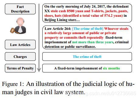
  • Topological Dependencies between Subtasks：子任务之间存在严格的顺序，如图1所示。具体流程：给定某案件的事实描述，大陆法系的法官首先确定与案件相关的法条（law articles），然后根据相关法条的说明确定指控罪名（charges）；基于上述结果，法官进一步确定处罚（penalty）和罚金（fines）。如何模仿法官的逻辑并建模子任务指甲剪的拓扑依赖将极大地影响审判预测的可信度和可解释性（creditability and interpretability）。
    
  • 由于特定任务的限制和忽视拓扑依赖性（the limitation of specific tasks and neglecting topological dependencies），传统工作无法解决这两个挑战。
• 文本方法：使用一个有向无环图（Directed Acyclic Graph，DAG）定义子任务之间的拓扑性的依赖关系，并提出一个统一的框架TOPJUDGE。具体来讲，给定事实描述的编码表示，TOPJUDGE根据拓扑顺序预测所有子任务的输出，并且某个特定子任务的输出将会影响其被依赖的子任务。
• 贡献：
  • 第一个将LJP的多个子任务统一到一个学习框架，此外，将LJP的子任务之间的依赖建立成DAG的形式并利用先验知识提升审判预测。
  • 提出统一多子任务的TOPJUDGE框架，和通过topological learning的审判预测。该模型可处理任何DAG依赖的子任务。
  • state-of-the-art 的结果

2、Related Work

2.1 Judgment Prediction

早期工作：通常侧重于使用数学和统计算法分析特定场景中的现有法律案例；

机器学习和文本挖掘技术 ：将其视为文本分类问题，

• 关注：从文本内容或案例注释（e.g., dates, terms, locations, and types）中提取有效的特征；
• 评价：这些方法利用浅层的文本特征和手动设计的因素，而两者都消耗大量人力，并且当应用于其他场景时会出现泛化的问题。

基于神经网络的方法

• 例如：基于注意力机制的神经网络等等

2.2 Multi-task Learning（MTL）

Multi-task learning (MTL) 旨在于通过同时解决相关任务，探索它们的共性和差异性（aims to exploit the commonalities and differences across relevant tasks by solving them at the same time），它可以在各种任务之间传递有用的信息，并已经有了广泛的应用。

常用思路：

• hard parameter sharing：sharing representations or some encoding layers among relevant tasks.
• soft parameter sharing：通常假设每个任务都有其特定的参数，不同任务中的参数之间的距离相近。
• 有部分工作关注：增加任务 或 处理无标签数据

本文工作中，我们介绍 拓扑(topological)学习框架 TOPJUDGE，用于处理 LJP 中的多个子任务。TOPJUDGE 不同于传统的 MTL 模型，这些模型侧重于如何在相关任务之间共享参数，TOPJUDGE 使用可扩展的 DAG 形式对这些子任务之间的显式依赖关系进行模型

3、Method

3.1 Problem Formulation

本文关注的是民法（civil law）中的 LJP 任务。

LJP 任务的定义：

• 假设一个案件的事实描述是一个单词序列 $\mathrm{x}=\{x_1,x_2,...,x_n\}$，其中 $n$ 表示 $\mathrm{x}$ 的长度，且每个单词 $x_i$ 都来自固定的词汇 $W$。
• 基于事实描述 $\mathrm{x}$，LJP $T$ 的任务是预测适用 law articles（法律条款）、charges（罪名指控）、term of penalty（处罚期限）、fines（罚款）等的判断结果。
• 形式上，假设 $T$ 包含 $|T|$ 个子任务，即 $T=\{t_1,t_2,...,t_{|T|}\}$，每个都是一个分类任务。对于第 $i$ 个子任务 $t_i\in T$，我们的目标是预测相应的结果 ${\mathrm{y}}_i\subseteq Y_i$，其中 $Y_i$ 是子任务特定标签集合。
• 以 charges prediction 的子任务为例：其对应的标签集合应该包括 Theft（偷窃）,Traffic Violation（交通违章）, Intentional Homicide（故意杀人）等等.

3.2 DAG Dependencies of Subtasks

我们假设 LJP 的多个子任务之间的依赖关系可形成 DAG。因此，任务列表 $T$ 应满足 topological constraints（拓扑约束）。

形式上：

• 使用记号 $t_i◃t_j$ 来定义第 $j$ 个子任务取决于第 $i$ 个子任务；$D_j=\{t_i|t_i◃t_j\}$ 定义依赖集合。
• 则任务列表 $T$ 需要满足以下约束：
  $$i<j,\forall (i,j)\in \{(i,j)|t_i\in D_j\}\text{\hspace{1em}(1)}$$

我们通过描述两个特殊情况，以展示公式的灵活性。

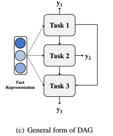
• （1）如图（a）所示，若不存在依赖，即 $D_j=\varnothing$，它对应于典型的 MTL setting，即我们同时对所有子任务进行预测。
  
• 如图（b）所示，若每个任务仅依赖于前一个的任务，即 $D_j=\{t_{j-1}\}$，它形成了一个顺序的学习过程。

3.3 Neural Encoder for Fact Descriptions

我们使用 a fact encoder 来生成 事实描述的向量表示，它作为 TOPJUDGE 的输入。此处使用一个基于 CNN 的 encoder。

将单词序列 $\mathrm{x}$ 作为输入，the CNN encoder 通过三个层（即lookup layer, convolution layer 和 pooling layer） 计算文本表示。

• Lookup：将 $\mathrm{x}$ 中的每个单词 $x_i$ 转换为 word embedding ${\mathrm{x}}_i\in {\mathbb{R}}^k$，其中 $k$ 表示 word embedding 的维度，则 word embedding 序列表示为
  $$\hat{\mathrm{x}}=\{{\mathrm{x}}_1,{\mathrm{x}}_2,...,{\mathrm{x}}_n\}\text{\hspace{1em}(2)}$$
• Convolution：卷积操作 涉及 卷积矩阵 $\mathrm{W}\in {\mathbb{R}}^{m\times (h\times k)}$，在该矩阵上应用 $m$ 个filter（其长度为 $h$），以生成 feature map，其中 ${\mathrm{x}}_{i:i+h-1}$ 是 $i$-th window 中 word embedding 的串联结果，$\mathrm{b}\in {\mathbb{R}}^m$ 是偏置向量。通过在每个window上运用conv操作，获得 $\mathrm{c}=\{c_1,...,c_{n-h+1}\}$
  $${\mathrm{c}}_i=\mathrm{W}\cdot {\mathrm{x}}_{i:i+h-1}+\mathrm{b}\text{\hspace{1em}(3)}$$
• Pooling：在 $c$ 的每个维度上应用 max pooling，并获得最终的事实表示 $\mathrm{d}=[d_1,d_2,...,d_m]$，计算公式如下：
  $$d_t=max(c_{1,t},...,c_{n-h+1,t}),\forall t\in [1,m]\text{\hspace{1em}(4)}$$

3.4 Judgment Predictor over DAG

基于 DAG 假设，我们获得一个有顺序的任务列表 $T^{\ast }=[t_1,t_2,...,t_{|T|}]$。对于每个任务 $t_j\in T$，我们的目标是 根据事实表示向量 $\mathrm{d}$ 及其所依赖任务的判断结果来预测其判断结果 ${\mathrm{y}}_j$。

为了预测，我们为每个任务使用特定的 LSTM cell，并按拓扑顺序获取每个任务的输出。更具体地说，对于每个任务 $t_j\in T$，通过三步获取其最终的判决结果，步骤：cell initialization, taskspecific representation, 和 prediction。

• Cell Initialization：$t_j$ 的预测结果将以 事实表示 $\mathrm{d}$ 和 所有依赖任务${\mathrm{y}}_k,\forall t_k\in D_j$ 的输出 为条件。因此，有
  $$\left[\begin{array}{c}\overline{{\mathrm{h}}_j}\\ \overline{{\mathrm{c}}_j}\end{array}\right]=\sum _{t_i\in D_j}({\mathrm{W}}_{i,j}\left[\begin{array}{c}{\mathrm{h}}_i\\ {\mathrm{c}}_i\end{array}\right])+{\mathrm{b}}_j\text{\hspace{1em}(5)}$$
  • 其中，${\mathrm{h}}_i$ 和 ${\mathrm{c}}_i$ 是 cell $t_i$ 的 hidden state(隐藏状态) 和memory cell (内存单元)。$\overline{{\mathrm{h}}_j}$ 和 $\overline{{\mathrm{c}}_j}$ 是 cell $t_j$ 的 initial hidden state(初始隐藏状态) 和memory cell (内存单元)。${\mathrm{W}}_{i,j}$和${\mathrm{b}}_j$是特定于 $t_i$ 和 $t_j$ 的变换矩阵和偏置矢量。
• Task-Specific Representation：
  • 输入：the fact representation $\mathrm{d}$, the initial hidden state $\overline{{\mathrm{h}}_j}$, 和 the initial memory cell $\overline{{\mathrm{c}}_j}$
  • 使用LSTM cell 处理输入：我们将 final hidden state ${\mathrm{h}}_j$ 作为任务 $t_j$ 的特定任务的表示。The last cell state ${\mathrm{c}}_j$ 用于构建接下来的任务的 the initial hidden state（初始隐含状态），如公式5所示。
• Prediction：在表示 ${\mathrm{h}}_j$ 上使用放射变换（affine transformation），然后应用 softmax，之后获得 the final prediction 如下：
  $${\hat{\mathrm{y}}}_j=\mathrm{s}\mathrm{o}\mathrm{f}\mathrm{t}\mathrm{m}\mathrm{a}\mathrm{x}({\mathrm{W}}_j^p{\mathrm{h}}_j+{\mathrm{b}}_j^p)\text{\hspace{1em}(6)}$$
  • 其中，${\mathrm{W}}_j^p$ 和 ${\mathrm{b}}_j^p$ 是特点任务 $t_j$ 的参数。
  • 优化：最小化 ${\hat{\mathrm{y}}}_j$ 和 ${\mathrm{y}}_j$ 之间的交叉熵，公式如下：
    $${\mathcal{L}}_j({\hat{\mathrm{y}}}_j,{\mathrm{y}}_j)=-\sum _{j=1}^{|Y_j|}{\mathrm{y}}_{j,k}\log ({\hat{\mathrm{y}}}_{j,k})\text{\hspace{1em}(7)}$$

3.5 Training

我们对每一个子任务使用交叉熵损失，并对所有任务的损失进行加权求和所有的损失来训练TOPJUDGE：
$$\mathcal{L}=\sum _{j=1}^{|T|}{\lambda }_j{\mathcal{L}}_j({\hat{\mathrm{y}}}_j,{\mathrm{y}}_j)\text{\hspace{1em}(8)}$$

• 其中，${\lambda }_j$ 是子任务 $t_j$ 的权重因子。

子任务的DAG依赖确保了本文模型是可微分的，并且可以以端到端的方式进行训练。在实践中，我们设置所有的 ${\lambda }_j=1$，使用 Adam 进行优化。为了防止过拟合，我们在fact representation上使用dropout。

4、Experiments

三个典型的子任务： law articles, charges, and the terms of penalty

4.1 Dataset Construction

数据集：CJO, PKU, 和 CAIL

• CJO：包含犯罪案件，数据来源 中国裁判文书网
• PKU：包含犯罪案件，数据来源 北大法宝
• CAIL：竞赛数据集，数据来源 中国裁判文书网
• 上述数据集文档有很好的结构和注释，易于提取 fact descriptions, applicable law articles, charges and the terms of penalty。

数据预处理：

• 数据过滤：对于存在多个被告和多项指控罪名的案件过滤，原因：本文关注点是子任务之间的拓扑性依赖的有效性；
• 数据过滤：对不常见的指控罪名（charges）和法律条款（law articles）的案件进行过滤，只保留频率大于100。
• 将 penalty 离散成非重叠的区间。

数据统计

4.2 Baselines

• TFIDF+SVM：特征提取 + 文本分类器
• CNN：多尺度核来 fact encoding、classification
• Hierarchical LSTM (HLSTM)：
• Fact-Law Attention Model（2017）：使用注意力机制捕捉fact描述和适用的law articles之间的交互作用来charge预测的神经网络模型；
• Pipeline Model (PM)：3 separate CNN classifiers for law articles, charges, and term of penalty，每个子任务的输入为 the concatenation of the fact representation 和 the embeddings for predicted labels of previous subtasks

4.3 Experimental Settings

分词：THULAC
预训练词向量：Skip-Gram model，embedding size = 200，frequency threshold = 25.
模型参数：the fact representation and task-specific representation = 256，maximum sentence length=128words，maximum document length=32sentences
超参数：learning rate（Adam）=$10^{-3}$，dropout=0.5，batch size=128，epochs=16
评价指标：accuracy (Acc.), macro-precision(MP), macro-recall (MR) 和 macro-F1 (F1)

4.4 Results and Analysis

子任务：law articles：$t_1$, charges：$t_2$, the terms of penalty：$t_3$

依赖设置：$D_1=\varnothing ,D_2=\{t_1\},D_3=\{t_1,t_2\}$，即charges依赖于law articles，the terms of penalty依赖于law articles和charges。

实验结果：

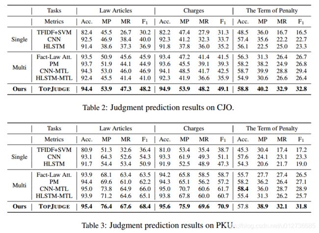
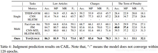
• 优于其他方法，体现本方法的有效性和鲁棒性；
• 与单任务模型相比：多任务模型利用相关子任务的相关性，并得到提升，体现子任务联合建模的重要性；
• charges and the terms of penalty的预测结果显著高于MTL方法，体现了LJP子任务的DAG依赖模型的合理性和重要性。

其他实验

研究：不同DAG依赖对结构性能的影响

5 Conclusion

In this paper, we focus on the task of legal judgment prediction (LJP) and address multiple subtasks of judgment predication with a topological learning framework. To be specific, we formalize the explicit dependencies over these subtasks in a DAG form, and propose a novel MTL framework, TOPJUDGE, by integrating the DAG dependencies. Experimental results on three LJP subtasks and three different datasets show that our TOPJUDGE outperforms all single-task baselines and conventional MTL models consistently and significantly.

探索思路：

• (1) 更多子任务、多场景案件（eg：多被告、多项指控罪名）下 TOPJUDGE 的有效性；
• (2) LJP + temporal factors（时间因素）