粒子滤波原理和MATLAB代码实现

理论基础¹：

(a) Prediction

• Use the transition equation to propagate the particles:

(b) Update

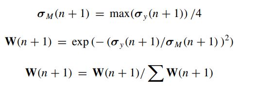
• Use the measurement equation to obtain measurements of the propagated particles and their standard deviations:

(in the case of our program, ym is obtained via simulation of the system, in real-time applications this value could be just the average of measurements).

• Evaluate the measurement PDF at the propagated particles. Then, normalize to obtain the weights. For instance:

(the weights have been denoted as pq(n) in the program)

• Resampling. Obtain new $\overline{p}x(n+1)$ from $a\overline{p}x(n+1)$using the normalized weights.

Note: Several resampling methods:

1、Multinomial Resampling

%Resampling (multinomial)
acq=cumsum(pq);
mm=1;
nr=sort(rand(1,Np)); %ordered random numbers (0, 1]
for ip=1:Np
    while(acq(mm)

2、Systematic Resampling

%Resampling (systematic)
acq=cumsum(pq);
cmb=linspace(0,1-(1/Np),Np)+(rand(1)/Np); %the "comb"
cmb(Np+1)=1;
ip=1; mm=1;
while(ip<=Np)
    if (cmb(ip)

3、 Stratified Resampling

%Resampling (stratified)
acq=cumsum(pq);
stf=zeros(1,Np);
nr=rand(1,Np)/Np;
j=1:Np;
stf(j)=nr(j)+((j-1)/Np); %(vectorized code)
stf(Np+1)=1;
ip=1; mm=1;
while(ip<=Np)
	if (stf(ip)

4、Residual Resampling

%Resampling (residual)
acq=cumsum(pq);
mm=1;
%preparation
na=floor(Np*pq); %repetition counts
NR=sum(na); %total count
Npr=Np-NR; %number of non-repeated particles
rpq=((Np*pq)-na)/Npr; %modified weights
acq=cumsum(rpq); %for the monomial part
%deterministic part
mm=1;
for j=1:Np
    for nn=1:na(j)
        Rpx(:,mm)=apx(:,j);
        mm=mm+1;
    end
end
%multinomial part:
nr=sort(rand(1,Npr)); %ordered random numbers (0, 1]
for j=1:Npr
    while(acq(mm)

一些比较研究表明，分层和系统重采样在滤波器估计和计算复杂度方面优于多项重采样。在残差重采样的情况下，大约一半的副本是确定的，另一半是随机的:这意味着更少的计算，但可以通过重新计算权重和算法的其他方面来补偿。部分实验证明，残差重采样的结果方差更小。

• Roughening

为了防止样本贫化，对后验粒子进行粗化处理[21,96]。添加一个零均值噪声，其方差正比于:

where n is the dimension of the space, k is a tuning parameter, and the j-th element of the vector M is:

where xm k (j) is the j-th component of the posterior particle xm k (which is a vector).

• Evaluate the mean of the set $\overline{p}x(n+1)$ This is the estimated state

代码实现¹：

%Particle filter example
%Radar monitoring of falling body
disp('please wait a bit');
%------------------------------------------
%Prepare for the simulation of the falling body
T=0.4; %sampling period
g=-9.81;
rho0=1.225; %air density, sea level
k=6705.6; %density vs. altitude constant
L=100; %horizontal distance radar<->object
L2=L^2;
Nf=100; %maximum number of steps
rx=zeros(3,Nf); %space for state record
tim=0:T:(Nf-1)*T; %time
%process noise
Sw=[10^5 0 0; 0 10^3 0; 0 0 10^2]; %cov
w11=sqrt(Sw(1,1)); w22=sqrt(Sw(2,2)); w33=sqrt(Sw(3,3));
w=[w11; w22; w33];
%observation noise
Sv=10^6; %cov.
v11=sqrt(Sv);
%------------------------------------------
%Prepare for filtering
%space for recording er(n), xe(n)
rer=zeros(3,Nf); rxe=zeros(3,Nf);
%------------------------------------------
%Behaviour of the system and the filter after initial state
x=[10^5; -5000; 400]; %initial state
xe=x; %initial estimation
%prepare particles
Np=1000; %number of particles
%reserve space
px=zeros(3,Np); %particles
apx=zeros(3,Np); %a priori particles
ny=zeros(1,Np); %particle measurements
vy=zeros(1,Np); %meas. dif.
pq=zeros(1,Np); %particle likelihoods
%particle generation
wnp=randn(3,Np); %noise (initial particles)
for ip=1:Np,
px(:,ip)=x+(w.*wnp(:,ip)); %initial particles
end
%system noises
wx=randn(3,Nf); %process
wy=randn(1,Nf); %output
nn=1;
while nn

结果：

参考：

---

1. Kalman Filter, Particle Filter and Other Bayesian Filters ↩︎ ↩︎