吴恩达《机器学习》——欠拟合与过拟合

数据集、源文件可以在Github项目中获得
链接: https://github.com/Raymond-Yang-2001/AndrewNg-Machine-Learing-Homework

1. 方差与偏差

在数学上，估计的偏差被定义为
$$\mathrm{bias}({\hat{\theta }}_{\mathrm{m}})=\mathbb{E}({\hat{\theta }}_{\mathrm{m}})-\theta$$
其中，期望作用在所有数据（看做从随机变量上采样得到的）上，$\theta$是作用于定义分布的$\theta$的真实值。如果$\mathrm{bias}({\hat{\theta }}_{\mathrm{m}})=0$，则说明这个估计是无偏估计；如果${\lim }_{m\to \infty }\mathrm{bias}({\hat{\theta }}_{\mathrm{m}})=0$，则称这个估计为渐进无偏估计。

除去偏差之外，我们有时还会考虑估计量的另一个性质是它作为数据样本的函数，期望的变化程度是多少。正如我们就可以计算估计量的期望来决定它的偏差，我们也可以计算出估计量的方差。
$$\mathrm{Var}(\hat{\theta })$$
当独立地从潜在的数据生成过程中进行重采样数据集时，我们希望估计的偏差和方差都比较小。在下面，我们会从方差和偏差的概念出发，讨论其在机器学习中与模型容量、过拟合、欠拟合的关系。

模型的容量、过拟合和欠拟合

机器学习的主要挑战之一就是算法必须在先前未知的输入上表现良好，这叫做模型的泛化能力。

在通常情况下，训练机器学习模型时，我们使用某个训练集，在训练集上的误差度量称作训练误差，优化算法的目标是降低训练误差，例如SGD算法。机器学习和优化的不同之处在与，机器学习还需要降低泛化误差，也成为测试误差。通常，我们会使用一个和训练集独立同分布的测试集来评估泛化误差。

我们可以总结影响机器学习算法好坏的因素如下：

1. 降低训练误差
2. 缩小训练误差和测试误差的差距

这其实对应了机器学习中两个关键的概念：欠拟合和过拟合。欠拟合指模型不能获得足够小的训练误差；过拟合置训练误差和测试误差之间的差距太大。

通过调整模型的容量，可以控制模型是否偏向过拟合还是欠拟合。模型的容量指的是模型拟合各种函数的能力，容量低的模型可能会出现欠拟合，容量过高的模型可能出现过拟合，因为模型拟合了一些不适合泛化的特征。

偏差和方差就度量了训练误差和泛化误差。

• 偏差度量了偏离真实函数或参数的误差的期望
• 方差度量了数据上任意特定采样导致的估计期望的偏差

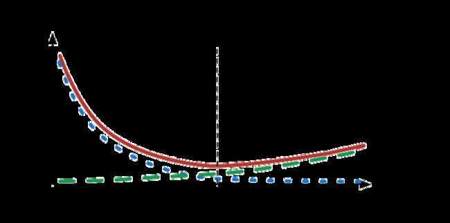
也就是说，偏差越大的模型，对应了训练误差偏大，模型欠拟合；方差越大的模型，对应了训练误差小，但是泛化误差远大于训练误差，模型过拟合。具体泛化误差曲线如下图所示：

2. Python代码实践

接下来，我们将使用线性回归的例子来进行代码实践。使用的数据集如下图所示：

直观的感觉是，我们需要拟合一个二次及以上的曲线才能很好的进行回归。接下来，将分别实现一次直线和多项式的拟合。
这里给出线性回归类和需要用到的函数

import numpy as np


def loss(pred, target):
    """
    MSE Loss
    :param pred: ndarray, (n_sample, n_feature), prediction
    :param target: ndarray, (n_sample, n_feature), target
    :return:
    """
    return np.sum(np.power((pred - target), 2)) / (2 * pred.shape[0])


def reg_loss(pred, target, theta, scale):
    """
    Regularized Loss (L2 regularize)
    :param pred:
    :param target:
    :param theta: parameters
    :param scale: lambda for regularize
    :return:
    """
    reg_term = theta.copy()  # (1, 2)
    reg_term[:, 0] = 0
    return loss(pred, target) + scale / (2 * pred.shape[0]) * reg_term.sum()


def gradient(x, pred, target):
    """
    Get gradient for model
    :param x:
    :param pred:
    :param target:
    :return:
    """
    # x(n,2)
    t = np.ones(shape=(x.shape[0], 1))
    x = np.concatenate((t, x), axis=1)
    # pred-target (n,1)
    # gradient (1,2)
    g = np.matmul((pred-target).T, x)
    return g / pred.shape[0]


def reg_gradient(x, pred, target, theta, scale):
    """
    Regularized gradient
    :param x:
    :param pred:
    :param target:
    :param theta:
    :param scale:
    :return:
    """
    g = gradient(x, pred, target)
    reg_term = theta.copy()
    reg_term[:, 0] = 0
    return g + (scale / pred.shape[0]) * reg_term


class LinearRegression:
    def __init__(self):
        self.theta = None

    def init_theta(self, shape):
        self.theta = np.zeros(shape)
        # self.theta = np.ones(shape)

    def optimize(self, g, lr):
        self.theta = self.theta - lr * g

    def load_parameters(self, parameters):
        self.theta = parameters

    def __call__(self, x, *args, **kwargs):
        #  x (n,2)
        t = np.ones(shape=(x.shape[0], 1))
        x = np.concatenate((t, x), axis=1)
        # (n,2)@(2,1)=(n,1)
        return x @ self.theta.T

2.1 拟合直线

from Bias import LinearRegression,loss,reg_loss,gradient,reg_gradient

epochs = 100
alpha = 0.05
regularize = False
scale = 0.1
x_norm = (train_x-train_x.mean(axis=0))/train_x.std(axis=0)
y_norm = (train_y-train_y.mean(axis=0))/train_y.std(axis=0)
train_loss = []
val_loss = []
test_loss = []
model = LinearRegression()
model.init_theta(shape=(1,2))
for epoch in range(epochs):
    pred = model(x_norm)
    g = reg_gradient(x_norm, pred, y_norm, model.theta, scale) if regularize else gradient(x_norm, pred, y_norm)
    model.optimize(g,alpha)

    theta = model.theta.copy()
    _theta = model.theta.copy()
    _theta[0, 1:] = _theta[0, 1:] / train_x.std(axis=0).T * train_y.std(axis=0)[0]
    _theta[0, 0] = _theta[0, 0] * train_y.std(axis=0)[0] + train_y.mean(axis=0)[0] - np.dot(_theta[0, 1:], train_x.mean(axis=0).T)
    # _theta[0, 0] = _theta[0, 0] - np.dot(_theta[0, 1:], train_x.mean(axis=0).T)
    model.load_parameters(_theta)
    pred = model(train_x)
    t_loss = reg_loss(pred,train_y,model.theta,scale) if regularize else loss(pred,train_y)
    train_loss.append(t_loss)
    pred_val = model(val_x)
    v_loss = reg_loss(pred_val,val_y,model.theta,scale) if regularize else loss(pred_val,val_y)
    val_loss.append(v_loss)

    test_pred = model(test_x)
    t_loss = reg_loss(test_pred, test_y, model.theta, scale)
    test_loss.append(t_loss)


    print("Epoch: {}/{}\tTrain Loss: {:.4f}\t\tVal Loss: {:.4f}\tTest Loss: {:.4f}".format(epoch, epochs,t_loss,v_loss, t_loss))
    model.load_parameters(theta)

# unscaling parameters
theta_f = np.zeros_like(model.theta)
theta_f[0, 1:] = model.theta[0, 1:] / train_x.std(axis=0).T * train_y.std(axis=0)[0]
theta_f[0, 0] = model.theta[0, 0] * train_y.std(axis=0)[0] + train_y.mean(axis=0)[0] - np.dot(theta_f[0, 1:], train_x.mean(axis=0).T)
theta_f

训练过程如下所示：

可以看到，在不使用正则化的时候，在训练的最后验证损失出现了轻微的上升，这其实是轻微的过拟合。但整体而言，训练损失、验证损失、泛化损失都在20-40的范围内，对于分布在0-60内的数据来说，这样的即使是训练损失也显得过大，这就证明模型的容量不足，存在严重的欠拟合现象，需要进一步提高模型容量来提升模型的拟合效果。

决策边界可视化如下图所示：

接下来，我们将使用多项式拟合。

2.2 拟合多项式

我们首先要对数据进行增强，这里将数据扩展为八个维度，对应1-8次方，并试图拟合一个八次多项式进行回归分析。

def feature_mapping(x, degree):
    # feature = np.zeros([x.shape[0],1])
    feature = [np.power(x[:,0],i) for i in range(1, degree+1)]
    return np.array(feature).T

train_x_map = feature_mapping(train_x,8)
val_x_map = feature_mapping(val_x,8)
test_x_map = feature_mapping(test_x, 8)
train_x_map

增强后的数据如下所示，以训练集为例：

进行训练

from Bias import LinearRegression,loss,reg_loss,gradient,reg_gradient

epochs = 200
alpha = 0.2
regularize = True
scale = 0
x_norm = (train_x_map-train_x_map.mean(axis=0))/train_x_map.std(axis=0)
y_norm = (train_y-train_y.mean(axis=0))/train_y.std(axis=0)
train_loss = []
val_loss = []
test_loss = []
model = LinearRegression()
model.init_theta(shape=(1,9))
for epoch in range(epochs):
    pred = model(x_norm)
    g = reg_gradient(x_norm, pred, y_norm, model.theta, scale) if regularize else gradient(x_norm, pred, y_norm)
    model.optimize(g,alpha)

    theta = model.theta.copy()
    _theta = model.theta.copy()
    _theta[0, 1:] = _theta[0, 1:] / train_x_map.std(axis=0).T * train_y.std(axis=0)[0]
    _theta[0, 0] = _theta[0, 0] * train_y.std(axis=0)[0] + train_y.mean(axis=0)[0] - np.dot(_theta[0, 1:], train_x_map.mean(axis=0).T)
    # _theta[0, 0] = _theta[0, 0] - np.dot(_theta[0, 1:], train_x_map.mean(axis=0).T)
    model.load_parameters(_theta)
    pred = model(train_x_map)
    t_loss = reg_loss(pred,train_y,model.theta,scale) if regularize else loss(pred,train_y)
    train_loss.append(t_loss)
    pred_val = model(val_x_map)
    v_loss = reg_loss(pred_val,val_y,model.theta,scale) if regularize else loss(pred_val,val_y)
    val_loss.append(v_loss)
    test_pred = model(test_x_map)
    t_loss = reg_loss(test_pred, test_y, model.theta, scale)
    test_loss.append(t_loss)

    print("Epoch: {}/{}\tTrain Loss: {:.4f}\t\tVal Loss: {:.4f}\tTest Loss: {:.4f}".format(epoch, epochs,t_loss,v_loss,t_loss))
    model.load_parameters(theta)


theta_f = np.zeros_like(model.theta)
theta_f[0, 1:] = model.theta[0, 1:] / train_x_map.std(axis=0).T * train_y.std(axis=0)[0]
theta_f[0, 0] = model.theta[0, 0] * train_y.std(axis=0)[0] + train_y.mean(axis=0)[0] - np.dot(theta_f[0, 1:], train_x_map.mean(axis=0).T)
theta_f

不进行正则化（正则化参数为0）

能看到在后半部分验证误差和测试误差明显加大，存在过拟合。

下面进行正则化，正则化参数为20。

可以看到，整体损失要显著大于上图，这说明出现严重的欠拟合，我们可以从决策边界看出来、

正则化参数为1

可以看到很明显地减轻了过拟合的现象。