神经网络 梯度下降
co-authored with Apurva Pathak
与Apurva Pathak合着
尝试梯度下降优化器 (Experimenting with Gradient Descent Optimizers)
Welcome to another instalment in our Deep Learning Experiments series, where we run experiments to evaluate commonly-held assumptions about training neural networks. Our goal is to better understand the different design choices that affect model training and evaluation. To do so, we come up with questions about each design choice and then run experiments to answer them.
欢迎来到我们的深度学习实验系列的另一部分,我们在其中进行实验以评估关于训练神经网络的普遍假设。 我们的目标是更好地了解影响模型训练和评估的不同设计选择。 为此,我们提出有关每个设计选择的问题,然后进行实验以回答这些问题。
In this article, we seek to better understand the impact of using different optimizers:
在本文中,我们试图更好地理解使用不同的优化器的影响:
- How do different optimizers perform in practice? 在实践中不同的优化器如何执行?
- How sensitive is each optimizer to parameter choices such as learning rate or momentum? 每个优化器对诸如学习率或动量之类的参数选择有多敏感?
- How quickly does each optimizer converge? 每个优化程序收敛的速度有多快?
- How much of a performance difference does choosing a good optimizer make? 选择一个好的优化器会对性能产生多大的影响?
To answer these questions, we evaluate the following optimizers:
为了回答这些问题,我们评估以下优化器:
- Stochastic gradient descent (SGD) 随机梯度下降(SGD)
- SGD with momentum 新元势头强劲
- SGD with Nesterov momentum 内斯托罗夫势头强劲的SGD
- RMSprop RMSprop
- Adam 亚当
- Adagrad 阿达格勒
- Cyclic Learning Rate 循环学习率
实验如何设置? (How are the experiments set up?)
We train a neural net using different optimizers and compare their performance. The code for these experiments can be found on Github.
我们使用不同的优化器训练神经网络并比较其性能。 这些实验的代码可以在Github上找到。
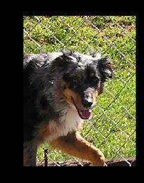
- Dataset: we use the Cats and Dogs dataset, which consists of 23,262 images of cats and dogs, split about 50/50 between the two classes. Since the images are differently-sized, we resize them all to the same size. We use 20% of the dataset as validation data (dev set) and the rest as training data. 数据集:我们使用“猫狗”数据集,该数据集由23,262张猫和狗的图像组成,在这两个类别之间划分为大约50/50。 由于图像的尺寸不同,因此我们将它们调整为相同的尺寸。 我们使用数据集的20%作为验证数据(开发集),其余作为训练数据。
- Evaluation metric: we use the binary cross-entropy loss on the validation data as our primary metric to measure model performance. 评估指标:我们使用验证数据上的二进制交叉熵损失作为衡量模型性能的主要指标。
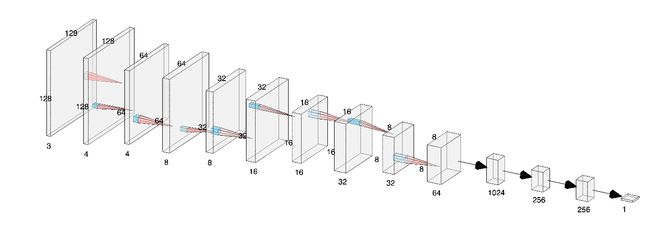
- Base model: we also define a base model that is inspired by VGG16, where we apply (convolution ->max-pool -> ReLU -> batch-norm -> dropout) operations repeatedly. Then, we flatten the output volume and feed it into two fully-connected layers (dense -> ReLU -> batch-norm) with 256 units each, and dropout after the first FC layer. Finally, we feed the result into a one-neuron layer with a sigmoid activation, resulting in an output between 0 and 1 that tells us whether the model predicts a cat (0) or dog (1). 基本模型:我们还定义了一个受VGG16启发的基本模型,我们在其中重复应用(卷积->最大池-> ReLU->批处理范数->退出)操作。 然后,我们将输出量展平,并将其馈入两个完全连接的层(密集-> ReLU->批处理规范),每个层具有256个单位,并在第一个FC层之后退出。 最后,我们将结果输入到具有S形激活的单神经元层中,从而得到0到1之间的输出,告诉我们该模型预测的是猫(0)还是狗(1)。
- Training: we use a batch size of 32 and the default weight initialization (Glorot uniform). The default optimizer is SGD with a learning rate of 0.01. We train until the validation loss fails to improve over 50 iterations. 培训:我们使用32批次大小和默认的重量初始化(Glorot统一)。 默认优化器为SGD,学习率为0.01。 我们进行训练,直到验证损失无法改善超过50次迭代为止。
随机梯度下降 (Stochastic Gradient Descent)
We first start off with vanilla stochastic gradient descent. This is defined by the following update equation:
我们首先从香草随机梯度下降开始。 这由以下更新方程式定义:
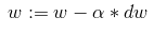
where w is the weight vector and dw is the gradient of the loss function with respect to the weights. This update rule takes a step in the direction of greatest decrease in the loss function, helping us find a set of weights that minimizes the loss. Note that in pure SGD, the update is applied per example, but more commonly it is computed on a batch of examples (called a mini-batch).
其中w是权重向量,dw是损失函数相对于权重的梯度。 此更新规则朝着损失函数最大减少的方向迈出了一步,从而帮助我们找到了使损失最小化的一组权重。 请注意,在纯SGD中,每个示例都会应用更新,但更常见的是,它是基于一批示例(称为迷你批处理)计算得出的。
学习率如何影响SGD? (How does learning rate affect SGD?)
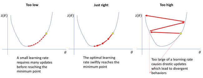
First, we explore how learning rate affects SGD. It is well known that choosing a learning rate that is too low will cause the model to converge slowly, whereas a learning rate that is too high may cause it to not converge at all.
首先,我们探讨学习率如何影响SGD。 众所周知,选择过低的学习速率会使模型收敛缓慢,而过高的学习速率可能会使模型完全收敛。
To verify this experimentally, we vary the learning rate along a log scale between 0.001 and 0.1. Let’s first plot the training losses.
为了通过实验验证这一点,我们沿0.001至0.1的对数刻度更改了学习率。 让我们首先绘制训练损失。

We indeed observe that performance is optimal when the learning rate is neither too small nor too large (the red line). Initially, increasing the learning rate speeds up convergence, but after learning rate 0.0316, convergence actually becomes slower. This may be because taking a larger step may actually overshoot the minimum loss, as illustrated in figure 4, resulting in a higher loss.
我们确实观察到,当学习率既不太小也不太大(红线)时,性能是最佳的。 最初,提高学习速率会加快收敛速度,但是在学习速率达到0.0316之后,收敛实际上会变慢。 这可能是因为采取更大的步骤实际上可能会超出最小损耗,如图4所示,从而导致更高的损耗。
Let’s now plot the validation losses.
现在让我们绘制验证损失。

We observe that validation performance suffers when we pick a learning rate that is either too small or too big. Too small (e.g. 0.001) and the validation loss does not decrease at all, or does so very slowly. Too large (e.g. 0.1) and the validation loss does not attain as low a minimum as it could with a smaller learning rate.
我们观察到,当选择的学习率太小或太大时,验证性能都会受到影响。 太小(例如0.001),验证损失根本不会减少,或者会非常缓慢地减少。 太大(例如0.1),并且验证损失无法达到学习率较小时的最小值。
Let’s now plot the best training and validation loss attained by each learning rate*:
现在,让我们来绘制每种学习率*可获得的最佳培训和验证损失:
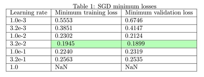
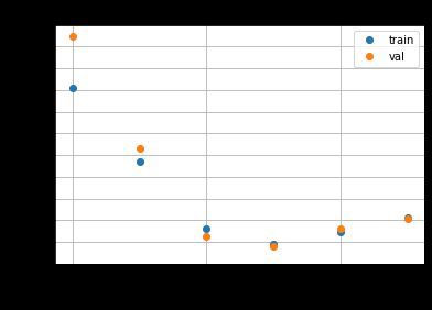
The data above confirm the ‘Goldilocks’ theory of picking a learning rate that is neither too small nor too large, since the best learning rate (3.2e-2) is in the middle of the range of values we tried.
上面的数据证实了“ Goldilocks”理论选择的学习率既不能太小也不能太大,因为最佳学习率(3.2e-2)处于我们尝试的值范围的中间。
*Typically, we would expect the validation loss to be higher than the training loss, since the model has not seen the validation data before. However, we see above that the validation loss is surprisingly sometimes lower than the training loss. This could be due to dropout, since neurons are dropped only at training time and not during evaluation, resulting in better performance during evaluation than during training. The effect may be particularly pronounced when the dropout rate is high, as it is in our model (0.6 dropout on FC layers).
*通常,由于模型之前没有看到验证数据,因此我们希望验证损失高于训练损失。 但是,我们在上面看到,验证损失有时会比训练损失低。 这可能是由于辍学造成的,因为神经元仅在训练时而不是在评估过程中被丢弃,从而导致评估期间的性能比训练期间更好。 当辍学率很高时,效果会特别明显,就像我们的模型一样(FC层上的辍学率为0.6)。
最佳SGD验证损失 (Best SGD validation loss)
- Best validation loss: 0.1899 最佳验证损失:0.1899
- Associated training loss: 0.1945 相关的训练损失:0.1945
- Epochs to converge to minimum: 535 收敛到最少的纪元:535
- Params: learning rate 0.032 参数:学习率0.032
SGD外卖 (SGD takeaways)
Choosing a good learning rate (not too big, not too small) is critical for ensuring optimal performance on SGD.
选择一个好的学习率(不要太大,不要太小)对于确保SGD的最佳性能至关重要。
动量的随机梯度下降 (Stochastic Gradient Descent with Momentum)
总览 (Overview)
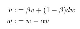
SGD with momentum is a variant of SGD that typically converges more quickly than vanilla SGD. It is typically defined as follows:
具有动量的SGD是SGD的变体,通常比原始SGD收敛更快。 通常定义如下:

Deep Learning by Goodfellow et al. explains the physical intuition behind the algorithm [0]:
Goodfellow等人的深度学习 。 解释了算法[0]背后的物理直觉:
Formally, the momentum algorithm introduces a variable v that plays the role of velocity — it is the direction and speed at which the parameters move through parameter space. The velocity is set to an exponentially decaying average of the negative gradient.
形式上,动量算法引入了一个变量v ,它起着速度的作用-它是参数在参数空间中移动的方向和速度。 速度设置为负梯度的指数衰减平均值。
In other words, the parameters move through the parameter space at a velocity that changes over time. The change in velocity is dictated by two terms:
换句话说,参数以随时间变化的速度在参数空间中移动。 速度的变化由两个术语决定:
- , the learning rate, which determines to what degree the gradient acts upon the velocity ,学习率,它决定梯度对速度的作用程度
- , the rate at which the velocity decays over time ,速度随时间衰减的速率
Thus, the velocity is an exponential average of the gradients, which incorporates new gradients and naturally decays old gradients over time.
因此,速度是梯度的指数平均值,其中合并了新的梯度并随着时间自然衰减了旧的梯度。
One can imagine a ball rolling down a hill, gathering velocity as it descends. Gravity exerts force on the ball, causing it to accelerate or decelerate, as represented by the gradient term * dw. The ball also encounters viscous drag, causing its velocity to decay, as represented by .
可以想象一个球从山上滚下来,随着球下降而加速。 重力在球上施加力,使球加速或减速,如梯度项 * dw所示 。 球还遇到粘性阻力,从而导致其速度衰减(以represented表示)。
One effect of momentum is to accelerate updates along dimensions where the gradient direction is consistent. For example, consider the effect of momentum when the gradient is a constant c:
动量的作用之一是沿梯度方向一致的维度加速更新。 例如,考虑梯度为常数c时动量的影响:

Whereas vanilla SGD would make an update of -c each time, SGD with momentum would accelerate over time, eventually reaching a terminal velocity that is 1/1- times greater than the vanilla update (derived using the formula for an infinite series). For example, if we set the momentum to =0.9, then the update eventually becomes 10 times as large as the vanilla update.
而香草SGD会使的更新- αc各自时间,SGD与动量会加快随着时间的推移,最终达到一个终极速度比所述香草更新一分之一-β倍的情况下(使用公式为一个无穷级数导出) 。 例如,如果将动量设置为 = 0.9,则更新最终将变为原始更新的10倍。
Another effect of momentum is that it dampens oscillations. For example, consider a case when the gradient zigzags and changes direction often along a certain dimension:
动量的另一个作用是抑制动量。 例如,考虑一种情况,其中渐变之字形并经常沿某个维度改变方向:
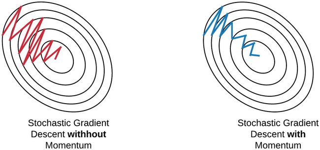
The momentum term dampens the oscillations because the oscillating terms cancel out when we add them into the velocity. This allows the update to be dominated by dimensions where the gradient points consistently in the same direction.
动量项抑制了振荡,因为当我们将它们添加到速度中时,振荡项会抵消。 这使得更新可以由梯度始终指向同一方向的尺寸决定。
实验 (Experiments)
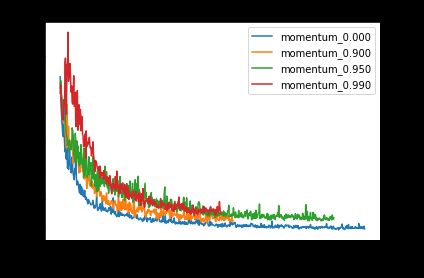
Let’s look at the effect of momentum at learning rate 0.01. We try out momentum values [0, 0.5, 0.9, 0.95, 0.99].
让我们看一下学习速率为0.01时动量的影响。 我们尝试了动量值[0,0.5,0.9,0.95,0.99]。
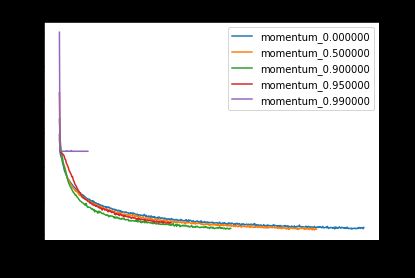
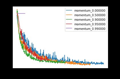
Above, we can see that increasing momentum up to 0.9 helps model training converge more quickly, since training and validation loss decrease at a faster rate. However, once we go past 0.9, we observe that training loss and validation loss actually suffer, with model training entirely failing to converge at momentum 0.99. Why does this happen? This could be because excessively large momentum prevents the model from adapting to new directions in the gradient updates. Another potential reason is that the weight updates become so large that it overshoots the minima. However, this remains an area for future investigation.
上图,我们可以看到将动量增加到0.9有助于模型训练更快收敛,因为训练和验证损失减少的速度更快。 但是,一旦超过0.9,我们就会发现训练损失和验证损失实际上受到了影响,模型训练完全无法收敛于动量0.99。 为什么会这样? 这可能是因为过大的动量会阻止模型在梯度更新中适应新的方向。 另一个潜在原因是权重更新变得如此之大,以至于超过了最小值。 但是,这仍然是未来研究的领域。
Do we observe the decrease in oscillation that is touted as a benefit of momentum? To measure this, we can compute an oscillation proportion for each update step — i.e. what proportion of parameter updates in the current update have the opposite sign compared to the previous update. Indeed, increasing the momentum decreases the proportion of parameters that oscillate:
我们是否观察到被吹捧为动量的优势而减少了振荡? 为了衡量这一点,我们可以为每个更新步骤计算一个振荡比例,即当前更新中参数更新与先前更新相比具有相反符号的比例。 的确,增加动量会降低振荡参数的比例:

What about the size of the updates — does the acceleration property of momentum increase the average size of the updates? Interestingly, the higher the momentum, the larger the initial updates but the smaller the later updates:
更新的大小如何-动量的加速属性会增加更新的平均大小吗? 有趣的是,动量越高,初始更新越大,但后来更新越小:
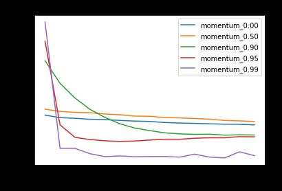
Thus, increasing the momentum results in taking larger initial steps but smaller later steps. Why would this be the case? This is likely because momentum initially benefits from acceleration, causing the initial steps to be larger. Later, the momentum causes oscillations to cancel out, which could make the later steps smaller.
因此,增加动量会导致采取较大的初始步骤,但采取较小的后续步骤。 为什么会这样呢? 这可能是因为动量最初会从加速中受益,从而导致初始步幅变大。 稍后,动量会抵消振荡,这可能会使后续步骤变小。
One data point that supports this interpretation is the distance traversed per epoch (defined as the Euclidean distance between the weights at the beginning of the epoch and the weights at the end of the epoch). We see that even though larger momentum values take smaller later steps, they actually traverse more distance:
支持该解释的一个数据点是每个历元遍历的距离(定义为历元开始时权重与历时结束时权重之间的欧几里得距离)。 我们看到,即使较大的动量值在后面走较小的步骤,它们实际上也会越过更多的距离:

This indicates that even though increasing the momentum values causes the later update steps to become smaller, the distance traversed is actually greater because the steps are more efficient — they do not cancel each other out as often.
这表明,即使增加动量值会导致以后的更新步骤变小,但由于这些步骤效率更高,因此经过的距离实际上更大,因为它们之间不会互相抵消。
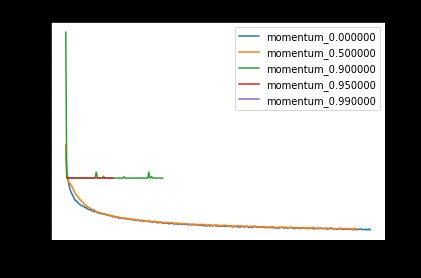
Now, let’s look at the effect of momentum on a small learning rate (0.001).
现在,让我们看一下动量对小学习率(0.001)的影响。


Surprisingly, increasing momentum on small learning rates helps it converge, when it didn’t before! Now, let’s look at a large learning rate.
出乎意料的是,以前所未有的速度提高小学习率的势头有助于它收敛! 现在,让我们看一下大学习率。
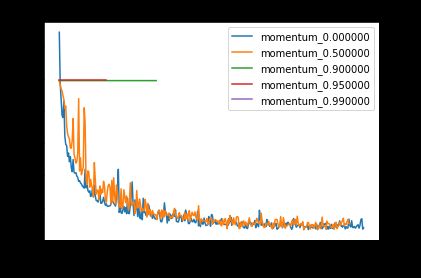
When the learning rate is large, increasing the momentum degrades performance, and can even result in the model failing to converge (see flat lines above corresponding to momentum 0.9 and 0.95).
当学习率很高时,增加动量会降低性能,甚至可能导致模型无法收敛(请参见上方的平线,对应于动量0.9和0.95)。
Now, to generalize our observations, let’s look at the minimum training loss and validation loss across all learning rates and momentums:
现在,为了概括我们的观察,让我们看一下所有学习率和动量下的最小训练损失和验证损失:

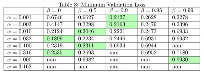
We see that the learning rate and the momentum are closely linked —the higher the learning rate, the lower the range of ‘acceptable’ momentum values (i.e. values that don’t cause the model training to diverge). Conversely, the higher the momentum, the lower the range of acceptable learning rates.
我们看到学习率和动量密切相关,学习率越高,“可接受”动量值(即不会引起模型训练发散的值)的范围越小。 相反,动力越高,可接受的学习率范围越小。
Altogether, the behavior across all the learning rates suggests that increasing momentum has an effect akin to increasing the learning rate. It helps smaller learning rates converge (Figure 14) but may cause larger ones to diverge (Figure 15). This makes sense if we consider the terminal velocity interpretation from Figure 9 — adding momentum can cause the updates to reach a terminal velocity much greater than than the vanilla updates themselves.
总的来说,所有学习率的行为都表明,增加动量的作用类似于提高学习率。 它有助于较小的学习率收敛(图14),但可能导致较大的学习率发散(图15)。 如果我们考虑图9中的终极速度解释,这是有道理的-增加动量可以导致更新达到终极速度,其速度要比原始更新本身大得多。
Note, however, that this does not mean that increasing momentum is the same as increasing the learning rate — there are simply some similarities in terms of convergence/divergence behavior between increasing momentum and increasing the learning rate. More concretely, as we can see in Figures 12 and 13, momentum also decreases oscillations, and front-loads the large updates at the beginning of training — we would not observe the same behaviors if we simply increased the learning rate.
但是请注意,这并不意味着增加动量与增加学习率相同–在增加动量和增加学习率之间在收敛/发散行为方面仅存在一些相似之处。 更具体地讲,如我们在图12和13中看到的那样,动量还减少了振荡,并且在训练开始时就将较大的更新提前加载了—如果仅提高学习速度,我们将不会观察到相同的行为。
动量的替代表达 (Alternative formulation of momentum)
There is another way to define momentum, expressed as follows:
还有另一种定义动量的方式,表示如下:
Andrew Ng uses this definition of momentum in his Deep Learning Specialization on Coursera. In this formulation, the velocity term is an exponentially moving average of the gradients, controlled by the parameter beta. The update is applied to the weights, with the size of the update controlled by the learning rate alpha. Note that this formulation is mathematically the same as the first formulation when expanded, except that all the terms are multiplied by 1-beta.
吴安德(Andrew Ng)在Coursera的深度学习专业课程中使用了这种动量定义。 在此公式中,速度项是由参数β控制的梯度的指数移动平均值。 将更新应用于权重,更新的大小由学习率alpha控制。 请注意,此公式在扩展时与第一个公式在数学上相同,只是所有术语均乘以1-beta。
How does this formulation of momentum work in practice?
这种动量公式在实践中如何起作用?

Surprisingly, using this alternative formulation, it looks like increasing the momentum actually slows down convergence!
出乎意料的是,使用这种替代公式,看起来增加势头实际上会减慢收敛速度!
Why would this be the case? This formulation of momentum, while dampening oscillations, does not enjoy the same benefit of acceleration that the other formulation does. If we consider a toy example where the gradient is always a constant c, we see that the velocity never accelerates:
为什么会这样呢? 这种动量公式在抑制振动的同时,没有像其他公式那样具有加速的好处。 如果我们考虑一个玩具示例,其中梯度始终为c ,则我们看到速度永远不会加速:

Indeed, Andrew Ng suggests that the main benefit of this formulation of momentum is not acceleration, but the fact that it dampens oscillations, allowing you to use a larger learning rate and therefore converge more quickly. Based on our experiments, increasing momentum by itself (in this formulation) without increasing the learning rate is not enough to guarantee faster convergence.
实际上,吴安德(Andrew Ng)表示,这种动量公式化的主要好处不是加速,而是抑制振荡的事实,使您可以使用较大的学习率,因此可以更快地收敛。 根据我们的实验,仅靠增加动量(在此公式中)而不增加学习率不足以保证更快的收敛。
有动力的SGD最佳验证损失 (Best validation loss on SGD with momentum)
- Best validation loss: 0.2046 最佳验证损失:0.2046
- Associated training loss: 0.2252 相关的训练损失:0.2252
- Epochs to converge to minimum: 402 收敛到最小限度的时代:402
- Params: learning rate 0.01, momentum 0.5 参数:学习率0.01,动量0.5
SGD带动力外卖 (SGD with momentum takeaways)
Momentum causes model training to converge more quickly, but is not guaranteed to improve the final training or validation loss, based on the parameters we tested.
根据我们测试的参数,动量会使模型训练收敛更快,但不能保证改善最终训练或验证损失。
The higher the learning rate, the lower the range of acceptable momentum values (ones where model training converges).
学习速率越高,可接受动量值(模型训练收敛的动量值)的范围越小。
Nesterov动量的随机梯度下降 (Stochastic Gradient Descent with Nesterov Momentum)
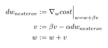
One issue with momentum is that while the gradient always points in the direction of greatest loss decrease, the momentum may not. To correct for this, Nesterov momentum computes the gradient at a lookahead point (w + velocity) instead of w. This gives the gradient a chance to correct for the momentum term.
动量的一个问题是,虽然梯度始终指向最大损耗减小的方向,但动量可能不会。 为了对此进行校正,涅斯捷罗夫动量计算的是先行点(w +速度)而不是w的梯度。 这使梯度有机会校正动量项。

To illustrate how Nesterov can help training converge more quickly, let’s look at a dummy example where the optimizer tries to descend a bowl-shaped loss surface, with the minimum at the center of the bowl.
为了说明Nesterov如何帮助更快地训练收敛,让我们看一个虚拟的示例,其中优化器尝试下降碗形的损失表面,使最小值位于碗的中心。

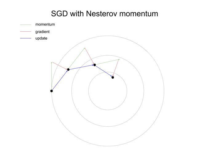
As the illustrations show, Nesterov converges more quickly because it computes the gradient at a lookahead point, thus ensuring that the update approaches the minimizer more quickly.
如图所示,Nesterov收敛更快,因为它可以在超前点计算梯度,从而确保更新更快地接近最小化器。
Let’s try out Nesterov on a subset of the learning rates and momentums we used for regular momentum, and see if it speeds up convergence. Let’s take a look at learning rate 0.001 and momentum 0.95:
让我们根据用于常规动量的学习速度和动量子集来测试Nesterov,看看它是否能加快收敛速度。 让我们看一下学习率0.001和动量0.95:

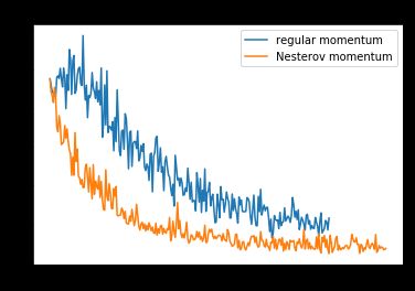
Here, Nesterov does indeed seem to speed up convergence rapidly! How about if we increase the momentum to 0.99?
在这里,涅斯捷罗夫的确确实确实在加快融合的速度! 如果将动量增加到0.99呢?

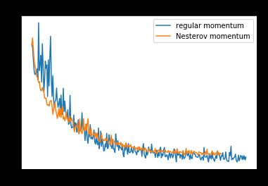
Now, Nesterov actually converges more slowly on the training loss, and though it initially converges more quickly on validation loss, it slows down and is overtaken by momentum after around 50 epochs.
现在,涅斯捷罗夫实际上在训练损失上收敛得较慢,尽管最初在验证损失上收敛得更快,但它变慢了,并在大约50个纪元后被动量所超越。
How should we measure speed of convergence over all the training runs? Let’s take the loss that regular momentum achieves after 50 epochs, then determine how many epochs Nesterov takes to reach that same loss. We define the convergence ratio as this number of epochs divided by 50. If it less than one, then Nesterov converges more quickly than regular momentum; conversely, if it is greater, then Nesterov converges more slowly.
我们应该如何衡量所有训练运行的收敛速度? 让我们以规则动量在50个纪元后达到的损失为例,然后确定Nesterov要达到相同的损失数个纪元。 我们将收敛率定义为该时期数除以50。如果小于1,则Nesterov的收敛速度要快于常规动量。 相反,如果更大,则涅斯捷罗夫收敛速度会更慢。

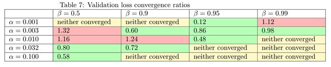
We see that in most cases (10/14) adding Nesterov causes the training loss to decrease more quickly, as seen in Table 5. The same applies to a lesser extent (8/12) for the validation loss, in Table 6.
我们看到,在大多数情况下(10/14),添加Nesterov会导致训练损失更快地减少,如表5所示。对于表象6中的验证损失,情况也是如此(8/12)较小。
There does not seem to be a clear relationship between the speedup from adding Nesterov and the other parameters (learning rate and momentum), though this can be an area for future investigation.
虽然添加Nesterov所带来的加速与其他参数(学习率和动量)之间似乎没有明确的关系,但是这可能是未来研究的领域。
Nesterov动量的SGD最佳验证损失 (Best validation loss on SGD with Nesterov momentum)
- Best validation loss: 0.2020 最佳验证损失:0.2020
- Associated training loss: 0.1945 相关的训练损失:0.1945
- Epochs to converge to minimum: 414 收敛到最小的时代:414
- Params: learning rate 0.003, momentum 0.95 参数:学习率0.003,动量0.95


内斯特罗夫动力外卖的SGD (SGD with Nesterov momentum takeaways)
Nesterov momentum computes the gradient at a lookahead point in order to account for the effect of momentum.
为了考虑动量的影响,涅斯捷罗夫动量会在先行点计算梯度。
Nesterov generally converges more quickly compared to regular momentum.
与常规动量相比,内斯特罗夫的收敛速度通常更快。
RMSprop (RMSprop)
The main idea of RMSProp is to divide the gradient by an exponential average of its recent magnitude. The update equations are as follows:
RMSProp的主要思想是将梯度除以最近幅度的指数平均值。 更新公式如下:
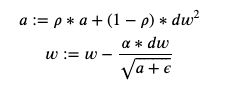
RMSprop tries to normalize the size of the updates across different weights — in other words, reducing the update size when the gradient is large, and increasing it when the gradient is small. As an example, consider a weight parameter where the gradients are [5, 5, 5] (and assume that =1). The denominator in the second equation is then 5, so the updates applied would be -[1, 1, 1]. Now, consider a weight parameter where the gradients are [0.5, 0.5, 0.5]; the denominator would be 0.5, giving the same updates -[1, 1, 1] as the previous case! In other words, RMSprop cares more about the direction (+ or -) of each weight than the magnitude, and tries to normalize the size of the update step for each of these weights.
RMSprop试图标准化不同权重上的更新大小-换句话说,当梯度大时减小更新大小,而当梯度小时增大更新大小。 例如,考虑一个权重参数,其中梯度为[5,5,5](并假定 = 1)。 那么第二个等式中的分母为5,因此应用的更新为-[1,1,1]。 现在,考虑权重参数,其中梯度分别为[0.5,0.5,0.5]; 分母将为0.5,与前面的情况相同,更新为[[1,1,1]! 换句话说,RMSprop更关心每个权重的方向(+或-),而不是大小,并尝试针对这些权重中的每个权重标准化更新步骤的大小。
This is different from vanilla SGD, which applies larger updates for weight parameters with larger gradients. Considering the above example where the gradient is [5, 5, 5], we can see that the resulting updates would be -[5, 5, 5], whereas for the [0.5, 0.5, 0.5] case the updates would be -[0.5, 0.5, 0.5]. Vanilla SGD thus is different from RMSprop in that the larger the gradient, the larger the update.
这不同于香草SGD,后者对具有较大梯度的权重参数应用较大的更新。 考虑上面的示例,其中梯度为[5,5,5],我们可以看到结果更新为-[5,5,5],而对于[0.5,0.5,0.5]情况,更新为- [0.5,0.5,0.5]。 因此,香草SGD与RMSprop的不同之处在于,梯度越大,更新越大。
学习率和rho如何影响RMSprop? (How do learning rate and rho affect RMSprop?)
Let’s try out RMSprop while varying the learning rate (default 0.001) and the coefficient (default 0.9). Let’s first try setting = 0 and vary the learning rate:
让我们尝试RMSprop,同时改变学习率(默认值0.001)和系数(默认值0.9)。 首先让我们设置 = 0并改变学习率:
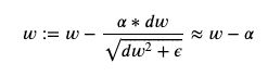
First lesson learned — don’t use RMSProp with =0! This results in the update being as follows:
第一堂课—不要在 = 0时使用RMSProp! 这导致更新如下:
Let’s try again over nonzero rho values. We first plot the train and validation losses for a small learning rate (1e-3).
让我们再次尝试非零的rho值。 我们首先以小学习率(1e-3)绘制火车和验证损失。
Increasing rho seems to reduce both the training loss and validation loss, but with diminishing returns — the validation loss ceases to improve when increasing rho from 0.95 to 0.99.
增加rho似乎可以减少训练损失和验证损失,但是收益却减少了-当rho从0.95增加到0.99时,验证损失不再改善。
Let’s now take a look at what happens when we use a larger learning rate.
现在让我们看一下使用较高学习率时会发生什么。


Here, the training and validation losses entirely fail to converge!
在这里,训练和验证损失完全无法收敛!
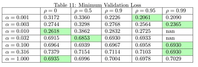
Let’s take a look at the minimum training and validation losses across all parameters:
让我们看一下所有参数的最小训练和验证损失:
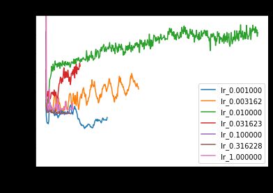
From the plots above, we find that once the learning rate reaches 0.01 or higher, RMSprop fails to converge.Thus, the optimal learning rate found here is around ten times as small as the optimal learning rate on SGD! One hypothesis is that the denominator term is much smaller than one, so it effectively scales up the update. Thus, we need to adjust the learning rate downward to compensate.
从上面的图中可以发现,一旦学习率达到0.01或更高,RMSprop就无法收敛,因此,此处找到的最佳学习率约为SGD最佳学习率的十倍! 一种假设是分母项远小于分母项,因此它有效地扩大了更新范围。 因此,我们需要向下调整学习率以进行补偿。
Regarding , we can see from the graphs above the RMS performs the best on our data with high values (0.9 to 1). Even though the Keras docs recommend using the default value of =0.9, it’s worth exploring other values as well — when we increased rho from 0.9 to 0.95, it substantially improved the best attained validation loss from 0.2226 to 0.2061.
关于,我们可以从上方的图表中看出,RMS具有高值(0.9到1),对我们的数据表现最佳。 即使Keras文档建议使用默认值 = 0.9,也值得探索其他值-当我们将rho从0.9增大到0.95时,它将获得的最佳验证损失从0.2226大大提高到0.2061。
RMSprop的最佳验证损失 (Best validation loss on RMSprop)
- Best validation loss: 0.2061 最佳验证损失:0.2061
- Associated training loss: 0.2408 相关的训练损失:0.2408
- Epochs to converge to minimum: 338 收敛到最少的纪元:338
- Params: learning rate 0.001, rho 0.95 参数:学习率0.001,rho 0.95
RMSprop外卖 (RMSprop takeaways)
RMSprop seems to work at much smaller learning rates than vanilla SGD (about ten times smaller). This is likely because we divide the original update (dw) by the averaged gradient.
RMSprop的学习速度似乎比香草SGD小得多(约小十倍)。 这可能是因为我们将原始更新(dw)除以平均梯度。
Additionally, it seems to pay off to explore different values of , contrary to the Keras docs’ recommendation to use the default value.
此外,探索 Ke的 不同值似乎 很有意义,这与Keras文档建议使用默认值相反。
亚当 (Adam)
Adam is sometimes regarded as the optimizer of choice, as it has been shown to converge more quickly than SGD and other optimization methods [1]. essentially a combination of SGD with momentum and RMSProp. It uses the following update equations:
亚当有时被认为是选择的优化器,因为它已被证明比SGD和其他优化方法收敛更快[1]。 本质上是SGD与动力和RMSProp的组合。 它使用以下更新方程式:
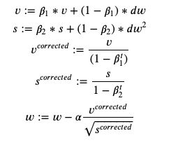
Essentially, we keep a velocity term similar to the one in momentum — it is an exponential average of the gradient updates. We also keep a squared term, which is an exponential average of the squares of the gradients, similar to RMSprop. We also correct these terms by (1 — beta); otherwise, the exponential average will start off with lower values at the beginning, since there are no previous terms to average over. Then we divide the corrected velocity by the square root of the corrected square term, and use that as our update.
本质上,我们保持类似于动量中的速度项-它是梯度更新的指数平均值。 我们还保留平方项,它是梯度平方的指数平均值,类似于RMSprop。 我们还将这些条款更正为(1-beta); 否则,指数平均值将在开始时以较低的值开始,因为没有先前的项可以进行平均。 然后,我们将校正后的速度除以校正后的平方项的平方根,并将其用作更新。
学习率如何影响亚当? (How does learning rate affect Adam?)
It has been suggested that the learning rate is more important than the β1 and β2 parameters, so let’s try varying the learning rate first, on a log scale from 1e-4 to 1:
有人建议,学习率比β1和β2参数更重要,因此让我们首先尝试以1e-4到1的对数刻度更改学习率:
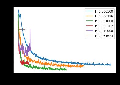
We did not plot learning rates above 0.03, since they failed to converge. We see that as we increase the learning rate, the training and validation loss decrease more quickly — but only up to a certain point. Once we increase the learning rate beyond 0.001, the training and validation loss both start to become worse. This could be due to the ‘overshooting’ behavior illustrated in Figure 4.
我们没有将学习率高于0.03,因为它们未能收敛。 我们看到,随着学习率的提高,训练和验证损失的减少速度会更快-但只能达到一定程度。 一旦我们将学习率提高到0.001以上,训练和验证损失就会开始变得越来越糟。 这可能是由于图4中所示的“超调”行为。
So, which of the learning rates is the best? Let’s find out by plotting the best validation loss of each one.
那么,哪个学习率是最好的? 让我们通过绘制每一个的最佳验证损失来找出答案。
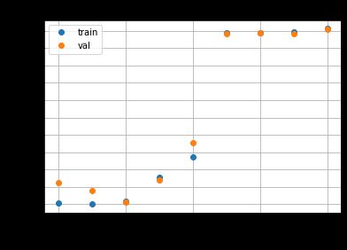
We see that the validation loss on learning rate 0.001 (which happens to be the default learning rate) seems to be the best, at 0.2059. The corresponding training loss is 0.2077. However, this is still worse than the best SGD run, which achieved a validation loss of 0.1899 and training loss of 0.1945. Can we somehow beat that? Let’s try varying β1 and β2 and see.
我们看到学习率0.001(恰好是默认学习率)的验证损失似乎是最好的,为0.2059。 相应的训练损失为0.2077。 但是,这仍然比最佳SGD运行更糟糕,后者的验证损失为0.1899,培训损失为0.1945。 我们能以某种方式击败它吗? 让我们尝试改变β1和β2看看。
β1和β2对亚当有何影响? (How do β1 and β2 affect Adam?)
We try the following values for β1 and β2:
我们为β1和β2尝试以下值:
beta_1_values = [0.5, 0.9, 0.95]
beta_2_values = [0.9, 0.99, 0.999]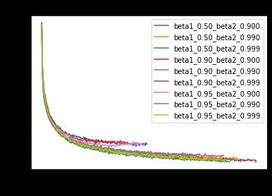
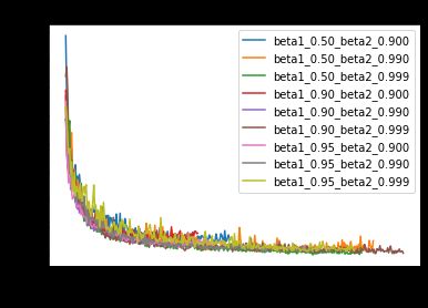
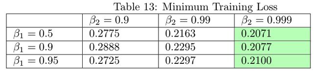
The best run is β1=0.5 and β2=0.999, which achieves a training loss of 0.2071 and validation loss of 0.2021. We can compare this against the default Keras params for Adam (β1=0.9 and β2=0.999), which achieves 0.2077 and 0.2059, respectively. Thus, it pays off slightly to experiment with different values of beta_1 and beta_2, contrary to the recommendation in the Keras docs — but the improvement is not large.
最佳运行是β1= 0.5和β2= 0.999,这将导致训练损失为0.2071,验证损失为0.2021。 我们可以将其与Adam的默认Keras参数(β1= 0.9和β2= 0.999)进行比较,后者分别达到0.2077和0.2059。 因此,与Keras文档中的建议相反,使用不同的beta_1和beta_2值进行试验会有所回报-但改进并不大。
Surprisingly, we were not able to beat the best SGD performance! It turns out that others have noticed that Adam sometimes works worse than SGD with momentum or other optimization algorithms [2]. While the reasons for this are beyond the scope of this article, it suggests that it pays off to experiment with different optimizers to find the one that works the best for your data.
令人惊讶的是,我们无法击败最佳SGD表现! 事实证明,其他人已经注意到,在使用动量或其他优化算法的情况下,Adam有时比SGD的工作效果更差[2]。 尽管造成这种情况的原因超出了本文的范围,但它表明尝试使用不同的优化器以找到最适合您数据的优化器是值得的。
最佳亚当验证损失 (Best Adam validation loss)
- Best validation loss: 0.2021 最佳验证损失:0.2021
- Associated training loss: 0.2071 相关的训练损失:0.2071
- Epochs to converge to minimum: 255 收敛到最小限度的时间:255
- Params: learning rate 0.001, β1=0.5, and β2=0.999 参数:学习率0.001,β1= 0.5,β2= 0.999
亚当外卖 (Adam takeaways)
Adam is not guaranteed to achieve the best training and validation performance compared to other optimizers, as we found that SGD outperforms Adam.
与其他优化程序相比,Adam无法保证获得最佳的培训和验证性能,因为我们发现SGD优于Adam。
Trying out non-default values for β1 and β2 can slightly improve the model’s performance.
试用β1和β2的非默认值可以稍微改善模型的性能。
阿达格勒 (Adagrad)
Adagrad accumulates the squares of gradients, and divides the update by the square root of this accumulator term.
Adagrad累加梯度的平方,然后用该累加项的平方根除以更新。
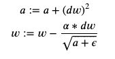
This is similar to RMSprop, but the difference is that it simply accumulates the squares of the gradients, without using an exponential average. This should result in the size of the updates decaying over time.
这类似于RMSprop,但不同之处在于,它仅累加了梯度的平方,而没有使用指数平均值。 这将导致更新的大小随时间衰减。
Let’s try Adagrad at different learning rates, from 0.001 to 1.
让我们以0.001到1的不同学习率尝试Adagrad。
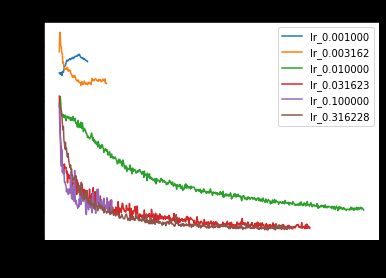
The best training and validation loss are 0.2057 and 0.2310, using a learning rate of 3e-1. Interestingly, if we compare with SGD using the same learning rates, we notice that Adagrad keeps pace with SGD initially but starts to fall behind in later epochs.
使用3e-1的学习率,最佳训练和验证损失为0.2057和0.2310。 有趣的是,如果我们使用相同的学习率与SGD进行比较,我们会注意到Adagrad最初与SGD保持同步,但在随后的时代开始落后。
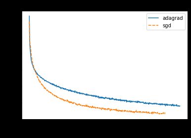

This is likely because Adagrad initially is dividing by a small number, since the gradient accumulator term has not accumulated many gradients yet. This makes the update comparable to that of SGD in the initial epochs. However, as the accumulator term accumulates more gradient, the size of the Adagrad updates decreases, and so the loss begins to flatten or even rise as it becomes more difficult to reach the minimizer.
这很可能是因为Adagrad最初会被一个小数除,因为梯度累加器项尚未累积很多梯度。 这使得更新在初始时期可与SGD相提并论。 但是,随着累加器项累积更多的梯度,Adagrad更新的大小会减小,因此,随着变得越来越难以达到最小化器,损耗开始趋于平坦甚至上升。
Surprisingly, we observe the opposite effect when we use a large learning rate (3e-1):
令人惊讶的是,当我们使用较大的学习率(3e-1)时,我们观察到相反的效果:
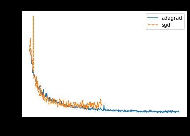
At large learning rates, Adagrad actually converges more quickly than SGD! One possible explanation is that while large learning rates cause SGD to take excessively large update steps, Adagrad divides the updates by the accumulator terms, essentially making the updates smaller and more ‘optimal.’
在较高的学习速度下,Adagrad实际上比SGD融合的速度更快! 一种可能的解释是,虽然较高的学习率会导致SGD采取过大的更新步骤,但Adagrad会将更新除以累加器项,从根本上使更新更小,更“最优”。
Let’s look at the minimum training and validation losses across all params:
让我们看一下所有参数的最小训练和验证损失:
We can see that the best learning rate for Adagrad, 0.316, is significantly larger than that for SGD, which was 0.03. As mentioned above, this is most likely because Adagrad divides by the accumulator terms, causing the effective size of the updates to be smaller.
我们可以看到,Adagrad的最佳学习率为0.316,大大高于SGD的0.03。 如上所述,这很可能是因为Adagrad除以累加器项,导致更新的有效大小较小。
Adagrad的最佳验证损失 (Best validation loss on Adagrad)
- Best validation loss: 0.2310 最佳验证损失:0.2310
- Associated training loss: 0.2057 相关的训练损失:0.2057
- Epochs to converge to minimum: 406 收敛到最小限度的时代:406
- Params: learning rate 0.312 参数:学习率0.312
阿达格勒外卖 (Adagrad takeaways)
Adagrad accumulates the squares of gradients, then divides the update by the square root of the accumulator term.
Adagrad累加梯度的平方,然后将更新除以累加器项的平方根。
The size of Adagrad updates decreases over time.
Adagrad更新的大小会随着时间的推移而减小。
The optimal learning rate for Adagrad is larger than for SGD (at least 10x in our case).
Adagrad的最佳学习率大于SGD(在我们的案例中至少为10倍)。
循环学习率 (Cyclic Learning Rate)
Cyclic Learning Rate is a method that lets the learning rate vary cyclically between a min and max value [4]. It claims to eliminate the need to tune the learning rate, and can help the model training converge more quickly.
循环学习率是一种使学习率在最小值和最大值之间周期性变化的方法[4]。 它声称不需要调整学习速率,并且可以帮助模型训练更快地收敛。
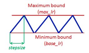
We try the cyclic learning rate with reasonable learning rate bounds (base_lr=0.1, max_lr=0.4), and a step size equal to 4 epochs, which is within the 4–8 range suggested by the author.
我们尝试使用合理的学习速率边界(base_lr = 0.1,max_lr = 0.4),且步长等于4个纪元,在作者建议的4–8范围内,以周期性学习率进行学习。

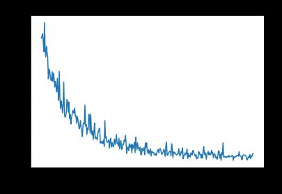
We observe cyclic oscillations in the training loss, due to the cyclic changes in the learning rate. We also see these oscillations to a lesser extend in the validation loss.
由于学习率的周期性变化,我们观察到训练损失中的周期性振荡。 我们还看到这些振荡在验证损失中的延伸较小。
最佳CLR培训和验证损失 (Best CLR training and validation loss)
- Best validation loss: 0.2318 最佳验证损失:0.2318
- Associated training loss: 0.2267 相关的训练损失:0.2267
- Epochs to converge to minimum: 280 收敛到最少的时代:280
- Params: Used the settings mentioned above. However, we may be able to obtain better performance by tuning the cycle policy (e.g. by allowing the max and min bounds to decay) or by tuning the max and min bounds themselves. Note that this tuning may offset the time savings that CLR purports to offer. 参数:使用上述设置。 但是,通过调整循环策略(例如,允许最大和最小边界衰减)或自行调整最大和最小边界,我们也许可以获得更好的性能。 请注意,此调整可能会抵消CLR声称可以节省的时间。
CLR外卖店 (CLR takeaways)
CLR varies the learning rate cyclically between a min and max bound.
CLR在最小和最大界限之间周期性地改变学习率。
CLR may potentially eliminate the need to tune the learning rate while attaining similar performance. However, we did not attain similar performance.
CLR可能会消除在达到类似性能的同时调整学习速率的需求。 但是,我们没有达到类似的性能。
比较方式 (Comparison)
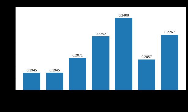
So, after all the experiments above, which optimizer ended up working the best? Let’s take the best run from each optimizer, i.e. the one with the lowest validation loss:
那么,经过以上所有实验,哪个优化程序最终表现最佳? 让我们从每个优化器中获得最佳运行,即验证损失最小的运行器:

Surprisingly, SGD achieves the best validation loss, and by a significant margin. Then, we have SGD with Nesterov momentum, Adam, SGD with momentum, and RMSprop, which all perform similarly to one another. Finally, Adagrad and CLR come in last, with losses significantly higher than the others.
出人意料的是,SGD的确最大程度地降低了验证损失。 然后,我们得到了具有Nesterov动量的SGD,Adam,具有动量的SGD和RMSprop,它们的性能都相似。 最后,Adagrad和CLR排名倒数第二,损失明显高于其他公司。
What about training loss? Let’s plot the training loss for the runs selected above:
训练损失呢? 让我们绘制以上所选跑步的训练损失:
Here, we see some correlation with the validation loss, but Adagrad and CLR perform better than their validation losses would imply.
在这里,我们看到了与验证损失的一些相关性,但是Adagrad和CLR的表现要好于其验证损失所暗示的。
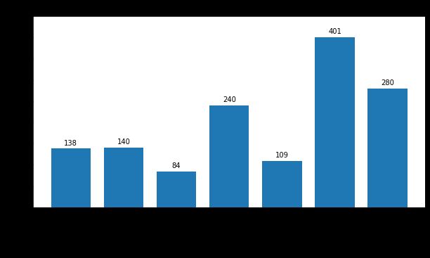
What about convergence? Let’s first take a look at how many epochs it takes each optimizer to converge to its minimum validation loss:
那么融合呢? 首先让我们看一下每个优化器收敛到最小验证损失所需的时间:
Adam is clearly the fastest, while SGD is the slowest.
亚当显然是最快的,而新币是最慢的。
However, this may not be a fair comparison, since the minimum validation loss for each optimizer is different. How about measuring how many epochs it takes each optimizer to reach a fixed validation loss? Let’s take the worst minimum validation loss of 0.2318 (the one achieved by CLR), and compute how many epochs it takes each optimizer to reach that loss.
但是,这可能不是一个公平的比较,因为每个优化程序的最小验证损失是不同的。 如何衡量每个优化器达到固定验证损失所需的时间? 让我们假设最差的最小验证损失为0.2318(CLR实现的损失),并计算每个优化程序达到该损失所花费的时间。
Again, we can see that Adam does converge more quickly to the given loss than any other optimizer, which is one of its purported advantages. Surprisingly, SGD with momentum seems to converge more slowly than vanilla SGD! This is because the learning rate used by the best SGD with momentum run is lower than that used by the best vanilla SGD run. If we hold the learning rate constant, we see that momentum does in fact speed up convergence:
再次,我们可以看到Adam确实比任何其他优化器都能更快地收敛到给定的损耗,这是其声称的优势之一。 出乎意料的是,具有势头的SGD收敛似乎比香草SGD慢! 这是因为具有动量运行的最佳SGD使用的学习速率低于最佳原始SGD运行的学习速率。 如果我们将学习率保持恒定,我们会发现动量确实会加速收敛:

As seen above, the best vanilla SGD run (blue) converges more quickly than the best SGD with momentum run (orange), since the learning rate is higher at 0.03 compared to the latter’s 0.01. However, when hold the learning rate constant by comparing with vanilla SGD at learning rate 0.01 (green), we see that adding momentum does indeed speed up convergence.
如上所示,最好的香草SGD运行(蓝色)比带有动量运行(橙色)的最佳SGD收敛更快,因为学习率比后者的0.01高,为0.03。 但是,当通过与学习速率为0.01(绿色)的香草SGD进行比较而使学习速率保持恒定时,我们看到增加动量确实确实会加快收敛。
为什么亚当无法击败香草SGD? (Why does Adam fail to beat vanilla SGD?)
As mentioned in the Adam section, others have also noticed that Adam sometimes works worse than SGD with momentum or other optimization algorithms [2]. To quote Vitaly Bushaev’s article on Adam, “after a while people started noticing that despite superior training time, Adam in some areas does not converge to an optimal solution, so for some tasks (such as image classification on popular CIFAR datasets) state-of-the-art results are still only achieved by applying SGD with momentum.” [2] Though the exact reasons are beyond the scope of this article, others have shown that Adam may converge to sub-optimal solutions, even on convex functions.
正如亚当部分中提到的那样,其他人也注意到亚当有时在使用动量或其他优化算法的情况下比SGD表现更差[2]。 引用Vitaly Bushaev关于Adam的文章,“一段时间后,人们开始注意到,尽管训练时间很长,但Adam在某些领域并没有收敛到最佳解决方案,因此对于某些任务(例如,流行的CIFAR数据集上的图像分类)来说仍然只有通过有力地应用SGD才能获得最先进的结果。” [2]尽管确切的原因不在本文讨论范围之内,但其他证据表明,即使在凸函数上,亚当也可能收敛于次优解。
结论 (Conclusions)
Overall, we can conclude that:
总的来说,我们可以得出以下结论:
You should tune your learning rate — it makes a large difference in your model’s performance, even more so than the choice of optimizer.
您应该调整学习速度-与选择优化器相比,它对模型性能的影响很大。
On our data, vanilla SGD performed the best, but Adam achieved performance that was almost as good, while converging more quickly.
根据我们的数据,香草SGD表现最好,但是Adam的表现几乎一样好,同时收敛速度更快。
It is worth trying out different values for rho in RMSprop and the beta values in Adam, even though Keras recommends using the default params.
即使Keras建议使用默认参数,也值得尝试使用RMSprop中的rho和Adam中的beta值不同的值。
翻译自: https://towardsdatascience.com/effect-of-gradient-descent-optimizers-on-neural-net-training-d44678d27060
神经网络 梯度下降