《Preservation of the Global Knowledge by Not-True Self Knowledge Distillation in Federated Learning》

《Preservation of the Global Knowledge by Not-True Self Knowledge Distillation in Federated Learning》

Abstract

1⃣️ Federated Learning’s convergence suffers from data heterogeneity.
2⃣️ forgetting could be the bottleneck of global convergence.
3⃣️ Continual Learning: fitting on biased local distribution shifts the feature on global distribution and results in forgetting of global knowledge.
4⃣️ Hypothesize that tackling down the forgetting in local training relives the data heterogeneity.
5⃣️ propose FedLSD(Federated Local Self-Distillation), which utilizes the global knowledge on locally available data.
6⃣️ extend FedLSD to FedLS-NTD, which only considers the not-true class signals to compensate noisy prediction of the global model.

Introduction

Federated Learning: train local models (need most computation), server aggregate local models to a single global model.
Base: FedAvg, heterogeneity is not resolved.
Local data (is not identically distributed) fails to represent the overall global distribution; makes the theoretical analysis difficult and degrades the FL algorithms’ performance.
CL (Continual Learning) causes catastrophic forgetting, because learning on the whole/different tasks.
FedAvg causes catastrophic forgetting(examine), because fitting on the biased local distribution -> forgetting of global knowledge.

tackle down forgetting -> heterogeneity decreased -> consistency increased.

Propose FedLSD

• preserve global knowledge
• local model self-distills the distributed global model’s prediction

FedLS-NTD

• by following not-true class signals noly

Forgetting global knowledge in FL

The prediction consistency degrades as data heterogeneity increases (less number of classes per client). As table 1 shows.
$Io{U}_{correct}=\frac{|D{G}_{correct}\cap A{G}_{correct}|}{|D{G}_{correct}\cup A{G}_{correct}|}$

How the representation on the global distribution changes during local training?
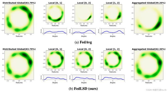
Map CIFAR-10 input data to 2-dimensional vectors and normalize them to be aligned on the unit hypersphere $S^1=\{x\in {\mathbb{R}}^2:\Vert x{\Vert }_2=1\}$. Then estimate the probability density function. The global model learned on homogeneous locals (i.i.d.) and heterogeneous locals with different local distributions.

Results show:
FedAvg: The feature vector from global model learned with homogeneous locals are uniformly distributed to hypersphere $S^1$. However, after local training, the entire feature region changed. The global model only reflects the feature regions where was dominant in the local models, and the knowledge of unseen classes is forgetten.
FedLSD: Preserving the knowledge on the global distribution prevents forgetting and relives the data heterogeneity problem.

Federated Local Self Distillation

Local self distillation

FedLSD: to preserve the global view on the local data, because the feature shifting occurs by fitting on the biased local distribution.
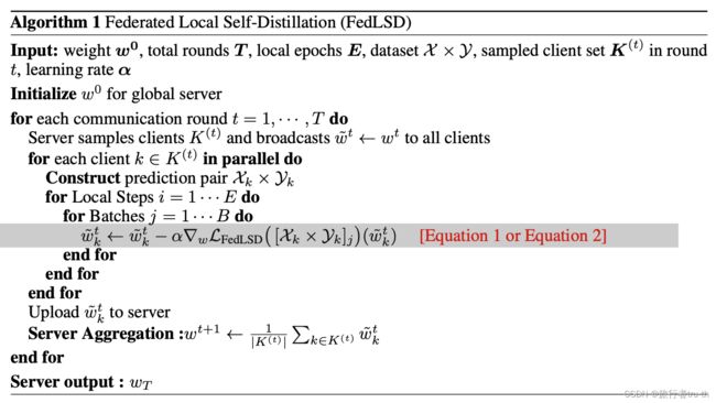
So, FedLSD conducts local-side self-distillation: using ${\mathcal{L}}_{FedLSD}$ and cross-entropy ${\mathcal{L}}_{CE}$.

$${\mathcal{L}}_{FedLSD}=(1-\beta )\cdot {\mathcal{L}}_{CE}(q,p_y)+\beta \cdot {\mathcal{L}}_{LSD}(q_{\tau },q_{\tau }^g)(0<\beta <1)\text{\hspace{1em}(1)}$$

where, $\{\begin{array}{l}{q}_{\tau }(c)=\frac{exp(z_c/\tau )}{{\sum }_{i=1}^{C}exp(z_i/\tau )};\\ q_{\tau }^g(c)=\frac{exp(z_c^g/\tau )}{{\sum }_{i=1}^{C}exp(z_i^g/\tau )};\end{array}$ , ${\mathcal{L}}_{LSD}(q_{\tau },q_{\tau }^g)=-{\sum }_{c=1}^C{q}_{\tau }^g(c)log(\frac{q_{\tau }(c)}{q_{\tau }^g(c)})$

where $q$,$q^g$ is the softmax probability of each local client model and global model at last round, and $p_y$ is the one-hot label.
C is the number of the classes
For distillation loss, the logins are divided by $\tau$ to soften the prediction probability.
${\mathcal{L}}_{LSD}$ is the KL-Divergence loss between local prediction and global prediction.

where FedLSD resembles memory-based CL algorithms, which exploits distillation loss to avoid forgetting by preserving the knowledge on old tasks. ->not allowed due to data privacy in FL.
Instead, the global model’s predictions can be utilized as a reference of the previous data distribution to induce a similar effect to that of using the episodic memory in CL.
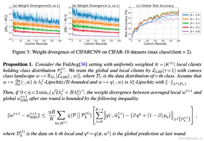
Proposition 1 implies that increasing $\beta$ in local objective reduces the weight divergence $||w^t-w_{GD}^t||$.

Local self not-true distillation

FedLSD is sub-optimal to prevent forgetting.
1⃣️ noisy global model’s predictions : FL updates with only a few local steps -> noisy -> KD-loss can’t good at tempreture softening -> teacher noisy should use a small temperature.
2⃣️ local information priority issues : information not included in the local distribution should have a higher priority to prevent forgetting.
3⃣️ FedLSD-NTD by distilling the global view on the relationship between not-true classes only.

FedLSD-NTD
$${\mathcal{L}}_{FedLSD-NTD}=(1-\beta )\cdot {\mathcal{L}}_{CE}(q,p_y)+\beta \cdot {\mathcal{L}}_{NTD}({\tilde{q}}_{\tau },{\tilde{q}}_{\tau }^g)(0<\beta <1)\text{\hspace{1em}(2)}$$

where, $\{\begin{array}{l}{\tilde{q}}_{\tau }(c)=\frac{exp(z_c/\tau )}{{\sum }_{i=1,i\ne y}^{C}exp(z_i/\tau )};\\ {\tilde{q}}_{\tau }^g(c)=\frac{exp(z_c^g/\tau )}{{\sum }_{i=1,i\ne y}^{C}exp(z_i^g/\tau )};\end{array}$ $(\forall x\ne y)$, ${\mathcal{L}}_{NTD}({\tilde{q}}_{\tau },{\tilde{q}}_{\tau }^g)=-{\sum }_{c=1,c\ne y}^C{\tilde{q}}_{\tau }^g(c)log(\frac{{\tilde{q}}_{\tau }(c)}{{\tilde{q}}_{\tau }^g(c)})$

Loss function
$${\mathcal{L}}_{LSD\to NTD}=(1-\beta )\cdot {\mathcal{L}}_{CE}(q,p_y)+\beta \cdot L(\lambda )$$
where$L(\lambda )=(1-\lambda )\cdot {\mathcal{L}}_{LSD}(q_{\tau },q_{\tau }^g)+\lambda \cdot {\mathcal{L}}_{NTD}(\widetilde{q_{\tau }},{\tilde{q}}_{\tau }^g)$

to improve the performance of the global model, an aggregated model should
1⃣️ preserve the correct prediction
2⃣️ discard the incorrect prediction of the previous global model.

Experiment

We evaluate our FedLSD and FedLS-NTD on various FL scenarios with data heterogeneity.

Performance on data heterogeneous FL scenarios

Compare the algorithms on different datasets to validate the efficacy of the proposed algorithms.

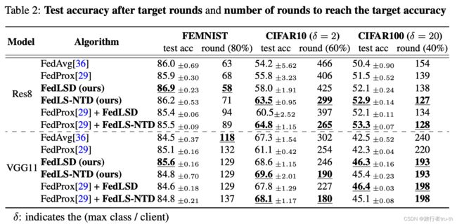
While FedLS-NTD generally performs better than FedLSD, the performance gap varies depending on the datasets and model architectures. We analyze that since FedLS-NTD learns not-true class relationships only, FedLSD may perform better when the prediction noise of the global model is not significant. We suggest that FedLS-NTD is more effective when the intensity of data heterogeneity is high, thereby following the global model possesses more risk to have biased distribution. For example, in FEMNIST datasets, almost all classes are included in the local data, but the hand-written data that belongs to the same class have different forms across the clients. In this case, FedLSD and FedLS-NTD show slow convergence in the early phase while they improve the final test accuracy.

We further investigate the performance by varying the data heterogeneity (Table 3) and sampling ratio (Table 4). The results show that the proposed algorithms significantly outperform the baselines in data heterogeneity cases.

Preservation of global knowledge

To empirically measure how well the global knowledge is preserved after local training, we examine the trained local models’ test accuracy on global distribution (Figure 7). If fitting on the local distribution preserves global knowledge, the trained local models could generalize well on the global distribution.

Analysis on feature similarity

Related work

Conclusion