CPT205-Computer Graphics(1)
文章目录
- 1. Introduction
-
- 1.1 Framebuffer
- 1.2 Raster display
- 2. Line Algorithms
-
- 2.1 DDA - Digital Differential Algorithm
- 2.2 Bresenham
- 2.3 Generation of circles
- 3. Transformation Pipeline and Geometric Transformations
-
- 3.1 Transformation pipeline
- 3.2 Types of geometric transformation
-
- 3.2.1 2D translation
- 3.2.2 2D rotation
- 3.2.3 2D scaling
- 3.2.4 2D reflection
- 3.2.5 2D shearing
- 3.2.6 2D homogeneous co-ordinates
- 3.2.7 3D transformation
- 3.3 OpenGL matrices
- 3.4 Current transformation matrix
-
- 3.4.1 CTM operations
- 3.4.2 Arbitrary Matrices
- 3.4.3 Matrix stacks
- 4. Viewing and Projection
-
- 4.1 Classic viewing & projection
- 4.2 Planar geometric projection
-
- 4.2.1 Perspective Projection
- 4.2.2 Parallel Projection
- 4.2.3 Orthographic Projection
- 4.2.4 Multiview Orthographic Projection
- 4.2.5 Axonometric Projections
- 4.2.6 Oblique Projection
- 4.3 Computer viewing and projection
-
- 4.3.1 3D viewing co-ordinate parameters
- 4.3.2 Orthogonal projection
- 4.3.3 Frustum perspective projection
- 4.3.4 Simple perspective projection
- 5. Parametric Curves and Surfaces
-
- 5.1 Parametric curves
- 5.2 Splines
-
- 5.2.1 Interpolation curve
- 5.2.2 Design curve
- 5.2.3 Local control
- 5.3 Types of parametric surface
-
- 5.3.1 Interpolation and design surfaces
- 6. 3D Modelling
-
- 6.1 3D modelling techniques
-
- 6.1.1 Wireframe
- 6.1.2 Surface
- 6.1.3 Solid
- 6.2 CSG
- 6.3 B-Rep
-
- 6.3.1 Types of B-Rep models
- 6.3.2 Euler’s law
- 6.3.4 Implementation of B-Rep models
- 6.3.5 Romulus and ACIS modellers
1. Introduction
‘Computer Graphics’ is concerned with all aspects of producing pictures or images using a computer. There are three closely related meanings, each representing a different perspective on the same thing.
- the images that you see on the computer screen
- the computer code that is used to create the images
- a mathematical model of the real-world (which is sometimes called the virtual world)
When working at the most advanced levels of Computer Graphics, the computer graphics specialist will
- create a virtual world
- implement the virtual world in computer code
- run the code to see life-like images on the computer screen
application areas:
- Display of information
- Design
- Simulation/modelling and animation
- User interfaces
- Virtual reality
1.1 Framebuffer
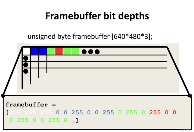
A block of memory, dedicated to graphics output, that holds the contents of what will be displayed.
Pixel
an element of the framebuffer.
bit depth
number of bits allocated per pixel in a buffer.
32 bits per pixel:
Video formats
- NTSC: 525 × 480 525\times 480 525×480, 30f/s, interlaced
- PAL: 625 × 480 625\times 480 625×480, 25f/s, interlaced
- VGA: 640 × 480 640\times 480 640×480, 60f/s, non-interlaced
- SVGA: 800 × 600 800\times 600 800×600, 60f/s, non-interlaced
- RGB: 3 independent video signals and synchronisation signal, vary in resolution and refresh rate
Interlaced: scan every other line at a time, or scan odd and even lines alternatively; the even scan lines are drawn and then the odd scan lines are drawn on the screen to make up one video frame.
1.2 Raster display
Cathode Ray Tubes (CRTs), most “tube” monitors you might see. Used to be very common, but big and bulky.

- Strong electrical fields and high voltage.
- Very good resolution
- Heavy, not flat
Liquid Crystal Displays (LCDs), there are two types transmissive (laptops, those snazzy new flat panel monitors) and reflective (wrist watches).
- Liquid crystal displays use small flat chips which change their transparency properties when a voltage is applied.
- LCD elements are arranged in an n x m array called the LCD matrix.
- The level of voltage controls grey levels.
- LCDs elements do not emit light; use backlights behind the LCD matrix.
- Colour is obtained by placing filters in front of each LCD element.
- Image quality dependent on viewing angle.
2. Line Algorithms
2.1 DDA - Digital Differential Algorithm
y = m x + b Δ y = m Δ x \begin{align}y&=mx+b\\\Delta y&=m\Delta x\end{align} yΔy=mx+b=mΔx
As we move along x x x by incrementing x x x, Δ x = 1 \Delta x=1 Δx=1, so Δ y = m \Delta y=m Δy=m
代码实现:
void DrawLine(int x0, int y0, int x1, int y1) {
	float dx = x1 - x0;
	float dy = y1 - y0;
	if (dx != 0) {
		float m = dy / dx;
		if (-1 <= m && m <= 1) {
			float y = y0;
			for (float x = x0; x <= x1; x++) {
				draw_pixel(x, round(y));
				y += m;
			}
		}
		else if (m < -1 || m > 1) {
			m = 1 / m;
			float x = x0;
			for (float y = y0; y <= y1; y++) {
				draw_pixel(round(x), y);
				x += m;
			}
		}
	}
	else {
		for (int y = min(y0, y1); y <= max(y0, y1); y++) {
			draw_pixel(x0, y);
		}
	}
}
针对任意斜率的 DDA:
void DrawLine(int x0, int x1, int y0, int y1) {
	int dx = x1 - x0;
	int dy = y1 - y0;
	int step = max(abs(dx), abs(dy));
	float deltaX = (float)dx / (float)step;
	float deltaY = (float)dy / (float)step;
	float x = x0;
	float y = y0;
	for (int i = 0; i <= step; i++) {
		draw_pixel(round(x), round(y));
		x += deltaX;
		y += deltaY;
	}
}
2.2 Bresenham
Bresenham 算法
2.3 Generation of circles
In Cartesian co-ordinates
( x − x c ) 2 + ( y − y c ) 2 = r 2 (x-x_c)^2+(y-y_c)^2=r^2 (x−xc)2+(y−yc)2=r2
The position of points on the circle circumference can be calculated by stepping along the x x x axis in unit steps from x c − r x_c-r xc−r to x c + r x_c+r xc+r and calculating the corresponding y y y value at each position as y = y c ± r 2 − ( x − x c ) 2 y=y_c\pm\sqrt{r^2-(x-x_c)^2} y=yc±r2−(x−xc)2
This method needs amount of computation. The spacing between plotted pixel positions is not uniform. This could be adjusted by interchanging x , y x,y x,y. However this simply increases the computation and processing required by the algorithm.
In polar co-ordinates
{ x = x c + r cos θ y = y c + r sin θ \begin{cases}x=x_c+r\cos\theta\\y=y_c+r\sin\theta\end{cases} {x=xc+rcosθy=yc+rsinθ
When a display is generated with these equations using a fixed angular step size, a circle is plotted with equally spaced points along the circumference. To reduce calculations, a large angular separation can be used between points along the circumference and connect the points with straight-line segments to approximate the circle path. For a more continuous boundary on a raster display, the angular step size can be set at 1 r \frac1r r1. This plots pixel positions that are approximately one unit apart.
Symmetry
Computations can be reduced by considering the symmetry of the circle. If the curve positions in the first quadrant are determined, the circle section in the second quadrant can be generated by noting that the two circle sections are symmetric with respect to the y y y axis. The same as x x x axis.
Taking this one step further, it can be noted that there is also symmetry between octants. Circle sections in adjacent octants within one quadrant are symmetric with respect to the 45° line dividing the two octants.

3. Transformation Pipeline and Geometric Transformations
3.1 Transformation pipeline
The Transformation Pipeline is the series of transformations (alterations) that must be applied to an object before it can be properly displayed on the screen.
The transformations can be thought of as a set of processing stages. If a stage is omitted, very often the object will not look correct. For example if the projection stage is skipped then the object will not appear to have any depth to it.
Once an object has passed through the pipeline it is ready to be displayed as either a wire-frame item or as a solid item.

Modelling Transformation: to place an object into the Virtual World.Viewing Transformation: to view the object from a different vantage point in the virtual world.Projection Transformation: to see depth in the object.Viewport Transformation: to temporarily map the volume defined by the “window of interest” plus the front and rear clipping planes into a unit cube. When this is the case, certain other operations are easier to perform.Device Transformation: to map the user defined “window of interest” (in the virtual world) to the dimensions of the display area.
We start when the object is loaded from a file and is ready to be processed. We finish when the object is ready to be displayed on the computer screen. You should be able to draw a picture of a simple object, say a cuboid, and show visually what happens to it as it passes through each pipeline stage.
3.2 Types of geometric transformation
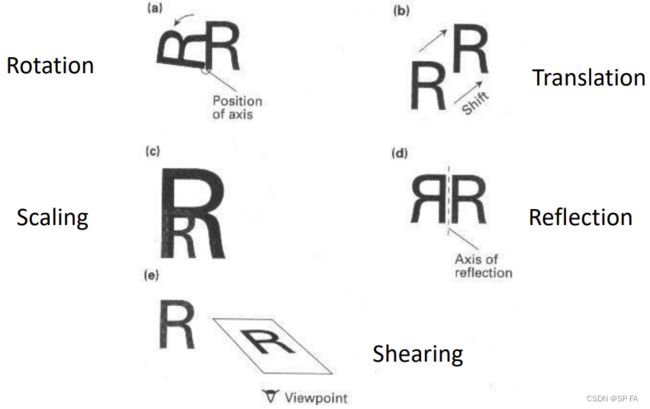
3.2.1 2D translation
Translating a point from P ( x , y ) P(x, y) P(x,y) to P ′ ( x ′ , y ′ ) P^\prime(x^\prime, y^\prime) P′(x′,y′) along T ⃗ \vec T T , that is: P ⃗ ′ = P ⃗ + T ⃗ \vec P^\prime=\vec P + \vec T P′=P+T
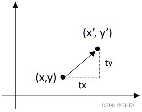 { x ′ = x + t x y ′ = y + t y \begin{cases}x^\prime=x+t_x\\y^\prime=y+t_y\end{cases} {x′=x+txy′=y+tyor [ x ′ y ′ ] = [ x y ] + [ t x t y ] \begin{bmatrix}x^\prime\\y^\prime\end{bmatrix}=\begin{bmatrix}x\\y\end{bmatrix}+\begin{bmatrix}t_x\\t_y\end{bmatrix} [x′y′]=[xy]+[txty]
3.2.2 2D rotation
3.2.3 2D scaling
P ⃗ ′ = P ⃗ ⋅ S \vec P^\prime=\vec P\cdot S P′=P⋅S
[ x ′ y ′ ] = [ s x 0 0 s y ] [ x y ] \begin{bmatrix}x^\prime\\y^\prime\end{bmatrix}=\begin{bmatrix}s_x&0\\0&s_y\end{bmatrix}\begin{bmatrix}x\\y\end{bmatrix} [x′y′]=[sx00sy][xy]
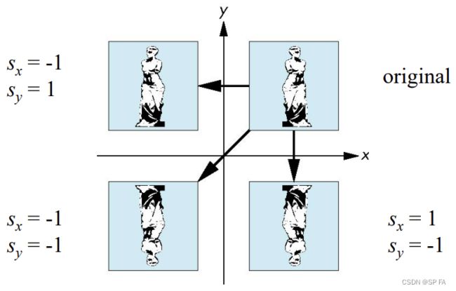
3.2.4 2D reflection
3.2.5 2D shearing
Consider simple shearing along the x axis.

[ x ′ y ′ ] = [ 1 cot θ 0 1 ] [ x y ] \begin{bmatrix}x^\prime\\y^\prime\end{bmatrix}=\begin{bmatrix}1&\cot\theta\\0&1\end{bmatrix}\begin{bmatrix}x\\y\end{bmatrix} [x′y′]=[10cotθ1][xy]
3.2.6 2D homogeneous co-ordinates
什么是齐次坐标?
By expanding 2 × 2 2\times2 2×2 matrices to 3 × 3 3\times3 3×3 matrices, homogeneous co-ordinates are used. A homogeneous parameter is applied so that each 2D position is represented with homogeneous co-ordinates (h·x, h·y, h). The homogeneous parameter has a non-zero value, and can be set to 1 for convenient use.
2D translation
[ x ′ y ′ 1 ] = [ 1 0 t x 0 1 t y 0 0 1 ] [ x y 1 ] \begin{bmatrix}x^\prime\\y^\prime\\1\end{bmatrix}=\begin{bmatrix}1&0&t_x\\0&1&t_y\\0&0&1\end{bmatrix}\begin{bmatrix}x\\y\\1\end{bmatrix} x′y′1 = 100010txty1 xy1
2D rotation
[ x ′ y ′ 1 ] = [ cos θ − sin θ 0 sin θ cos θ 0 0 0 1 ] [ x y 1 ] \begin{bmatrix}x^\prime\\y^\prime\\1\end{bmatrix}=\begin{bmatrix}\cos\theta&-\sin\theta&0\\\sin\theta&\cos\theta&0\\0&0&1\end{bmatrix}\begin{bmatrix}x\\y\\1\end{bmatrix} x′y′1 = cosθsinθ0−sinθcosθ0001 xy1
2D scaling
[ x ′ y ′ 1 ] = [ s x 0 0 0 s y 0 0 0 1 ] [ x y 1 ] \begin{bmatrix}x^\prime\\y^\prime\\1\end{bmatrix}=\begin{bmatrix}s_x&0&0\\0&s_y&0\\0&0&1\end{bmatrix}\begin{bmatrix}x\\y\\1\end{bmatrix} x′y′1 = sx000sy0001 xy1
2D shearing
[ x ′ y ′ 1 ] = [ 1 cot θ 0 0 1 0 0 0 1 ] [ x y 1 ] \begin{bmatrix}x^\prime\\y^\prime\\1\end{bmatrix}=\begin{bmatrix}1&\cot\theta&0\\0&1&0\\0&0&1\end{bmatrix}\begin{bmatrix}x\\y\\1\end{bmatrix} x′y′1 = 100cotθ10001 xy1
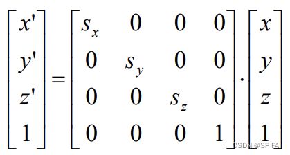
3.2.7 3D transformation
3.3 OpenGL matrices
In OpenGL matrices are part of the state.
- model-view: GL_MODELVIEW
- projection: GL_PROJECTION
- texture: GL_TEXTURE
- color: GL_COLOR
Single set of functions for manipulation. Select which to be manipulated by
- glMatrixMode(GL_MODELVIEW);
- glMatrixMode(GL_PROJECTION);
3.4 Current transformation matrix
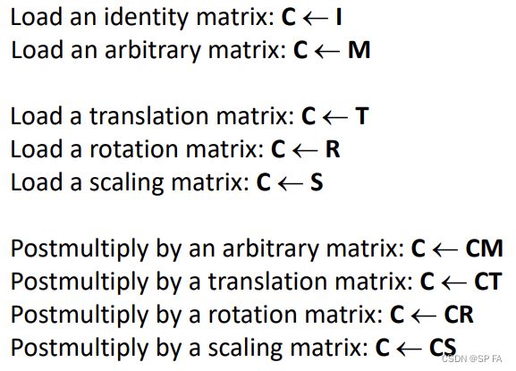
Conceptually there is a 4 × 4 4\times4 4×4 homogeneous coordinate matrix, the current transformation matrix (CTM) that is part of the state and is applied to all vertices that pass down the pipeline. The CTM is defined in the user program and loaded into a transformation unit. The CTM can be altered either by loading a new CTM or by postmutiplication.
OpenGL has a model-view and a projection matrix in the pipeline which are concatenated together to form the CTM. The CTM can manipulate each by first setting the correct matrix mode.
3.4.1 CTM operations
3.4.2 Arbitrary Matrices
glLoadMatrixf(m) / glMultMatrixf(m)
m m m is a one-dimension array of 16 elements which are the components of the desired 4 × 4 4\times4 4×4 matrix stored by columns. In glMultMatrixf, m multiplies the existing matrix on the right.
3.4.3 Matrix stacks
CTM is not just one matrix but a matrix stack with the “current” at top.
In many situations we want to save transformation matrices for use later
- Traversing hierarchical data structures
- Avoiding state changes when executing display lists
We can also access matrices (and other parts of the state) with query functions
- glGetIntegerv
- glGetFloatv
- glGetBooleanv
- glGetDoublev
- glIsEnabled
For matrices, we use as
double m[16];
glGetFloatv(GL_MODELVIEW, m);
4. Viewing and Projection
4.1 Classic viewing & projection
Viewing requires three basic elements:
- One or more objects
- A viewer with a projection surface
- Projectors that go from the objects to the projection surface.
Classical views are based on the relationship among hese elements. Each object is constructed from flat principal faces.
4.2 Planar geometric projection
Standard projections project onto a plane. Projectors are lines that either converge at a centre of projection or are parallel. Such projections preserve lines but not necessarily angles.
Non-planar projections are needed for applications such as map construction.
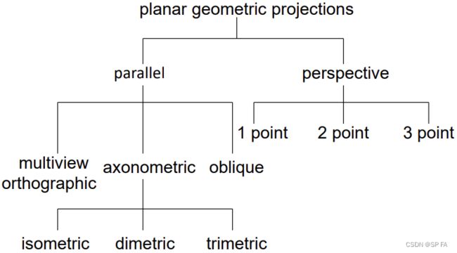
4.2.1 Perspective Projection
Perspective projection generates a view of 3-dimensional scene by projecting points to the view plane along converging paths, causing the objects farther from the viewing position to be displayed smaller than the objects of the same size that are nearer to the viewing position.
A scene generated using perspective projection appears more realistic since this is the way that human eyes and cameras form images.
Vanishing Points
Parallel lines (not those parallel to the projection plane) on the object converge at a single point in the projection (the vanishing point).
Advantages
- Objects further from the viewer are projected smaller than the same sized objects closer to the viewer (diminution) (Looks realistic)
Disadvantages
- Equal distances along a line are not projected into equal distances (non-uniform foreshortening).
- Angles preserved only in planes parallel to the projection plane.
- More difficult to construct by hand than parallel projections (but not more difficult by computer).
4.2.2 Parallel Projection
This method projects points on the object surface along parallel lines.
It is usually used in engineering and architecture drawings to represent an object with a set of views showing accurate dimensions.
4.2.3 Orthographic Projection
The projectors are orthogonal to projection surface.
4.2.4 Multiview Orthographic Projection
The projection plane is parallel to the principal face. Usually form front, top and side views.

Advantages
- Preserves both distances and angles
- Shapes preserved
- Can be used for measurements
Disadvantages
- Cannot see what object really looks like because many surfaces are hidden from the view
4.2.5 Axonometric Projections
Allow projection plane to move relative to the object.
轴测投影图详解
Advantages
- Lines are scaled (foreshortened) but can find scaling factors
- Lines preserved but angles are not
- Can see three principal faces of a box-like object
Disadvantages
- Some optical illusions possible
- Does not look real because far objects are scaled the same as near objects
4.2.6 Oblique Projection
Arbitrary relationship between projectors and projection plane.
Advantages
- Can pick the angles to emphasise a particular face
- Angles in faces parallel to the projection plane are preserved while we can still see “around” side.
Disadvantages
- In the physical world, we cannot create oblique projections with a simple camera; possible with bellows camera or special lens (architectural)
轴测投影和斜投影的区别
4.3 Computer viewing and projection
There are three aspects of the viewing process, all of which are implemented in the pipeline:
- Positioning the camera. Setting the model-view matrix
- Selecting a lens. Setting the projection matrix
- Clipping. Setting the view volume
4.3.1 3D viewing co-ordinate parameters
A world co-ordinate position P 0 ( x 0 , y 0 , z 0 ) P_0(x_0, y_0, z_0) P0(x0,y0,z0) is selected as the viewing origin (called view point, viewing position, eye position or camera position).
The view plane can then be defined with a normal vector, which is the viewing direction, usually the negative z view z_\text{view} zview axis.
The viewing plane is thus parallel to the x view − y view x_\text{view}-y_\text{view} xview−yview plane.
The direction from a reference point to the viewing point can be taken as the viewing direction (vector), and the reference point ( x ref , y ref , z ref ) (x_\text{ref}, y_\text{ref}, z_\text{ref}) (xref,yref,zref) is termed the look-at point.
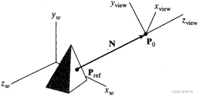
Once the viewing plane normal vector N ⃗ \vec N N is defined, the direction for view-up vector V ⃗ \vec V V can be set to establish the positive x view x_\text{view} xview axis. Since N ⃗ \vec N N defines the direction for z view z_\text{view} zview, V ⃗ \vec V V must be perpendicular to N ⃗ \vec N N (i.e. parallel to the x view − y view x_\text{view}-y_\text{view} xview−yview plane).
But it is generally difficult to determine V ⃗ \vec V V precisely, and viewing routines typically adjust the user defined value of V ⃗ \vec V V (e.g. projecting it onto a plane perpendicular to v e c N vec N vecN).
Any direction can be used for V ⃗ \vec V V as long as it is not parallel to N ⃗ \vec N N.
4.3.2 Orthogonal projection
Orthogonal (orthographic) projection is a transformation of object descriptions to a view plane along lines parallel to the view-plane normal vector N ⃗ \vec N N.
It is often used to produce the front, side and top views of an object.


4.3.3 Frustum perspective projection

By adding near and far clipping planes that are parallel to the viewing plane, parts of the infinite perspective view volume are chopped off to form a truncated pyramid or frustum. These clipping planes can be optional for some systems.
The near and far clipping planes can be used simply to enclose objects to be displayed. The near clipping plane can be used to take out large objects close to the viewing plane, which could be projected into unrecognisable shapes in the clipping window. Likewise, the far clipping plane can cut out objects that may be projected to small blots.
Some systems restrict the placement of the viewing plane relative to the near and far planes, and other systems allow it to be placed anywhere except at the position of the viewing origin (view point, viewing position, eye position or camera position).
If the viewing plane is behind the projection reference point, objects are inverted on the view plane.
If the viewing plane is behind the objects, the objects are simply enlarged as they are projected away.
When the projection reference point is very far away from the view plane, a perspective projection approaches to a parallel projection.
4.3.4 Simple perspective projection
Let the centre of projection at the origin, projection plane is z = d , d < 0 z=d,d<0 z=d,d<0
Consider the top and side views:

5. Parametric Curves and Surfaces
Parametric surfaces are surfaces that are usually parameterised by two independent variables. By parameterisation, it is relatively easy to represent surfaces that are self-intersecting or non-orientable.
It is impossible to represent many of these surfaces by using implicit functions. Even where implicit functions exist for these surfaces, the tessellated representation is often incorrect.
5.1 Parametric curves
A curve in a 2D surface is defined as: x = x ( t ) y = y ( t ) s . t . t ∈ [ 0 , 1 ] x=x(t)\\y=y(t)\\s.t.~t\in[0,1] x=x(t)y=y(t)s.t. t∈[0,1]
In this way the curve is well defined, each value of t t t in [ 0 , 1 ] [0,1] [0,1] defining one and only one point. The curve description will not change when rotation occurs.
Implicit representation: y = a 0 + a 1 x y=a_0+a_1x y=a0+a1x
Parametric (explicit) representation: x = x 1 + t ( x 2 − x 1 ) y = y 1 + t ( y 2 − y 1 ) x=x_1+t(x_2-x_1)\\y=y_1+t(y_2-y_1) x=x1+t(x2−x1)y=y1+t(y2−y1)
Implicit representation: x 2 + y 2 = r 2 x^2+y^2=r^2 x2+y2=r2
Parametric equation: x = r cos ( 360 t ) y = r sin ( 360 t ) x=r\cos(360t)\\y=r\sin(360t) x=rcos(360t)y=rsin(360t)
5.2 Splines
A curve description should be used, which allows rapid computation (i.e. functions such as sin, cos, exp, log, and so on should be avoided), a polynomial can therefore be used. For interpolation, if there are k k k points, then n = k – 1 n = k – 1 n=k–1 must be chosen, in order to find the correct values for ai.
Low-degree polynomial curves
Polynomials have to be used for efficiency. High-degree polynomials are not suitable because of their behaviour. For curves of a large number of points
- they can be broken into small sets
- a low-degree polynomial is put through each set
- these individual curves (cubics) are joined up smoothly
A spline curve consists of individual components, joined together smoothly, looking like a continuous smooth curve.
Different types of continuity exist and the following are generally required
- continuity of the curve (no breaks)
- continuity of tangent (no sharp corners)
- continuity of curvature (not essential but avoids some artefact from lighting)
Each component is a low-degree polynomial, and for these continuities, cubic polynomials are generally needed.
5.2.1 Interpolation curve
An interpolation curve defines the exact position (point) that the curve must pass through, e.g. in a keyframe animation, an object must be at a particular point at a particular time.
The shape of the interpolation curve depends on the data points provided.
5.2.2 Design curve
A design curve defines the general behaviour of the curve, e.g. what the curve should look like, and tuning the shape is often needed. The method is often used by designers.
The shape of the design curve depends on the control points, which do not lie on the curve, but allow adjustment of the shape by moving the points.
5.2.3 Local control
When a curve is designed, if one part is done, it would be preferred to keep its current shape when another part of the curve is adjusted. So the adjustment should influence only a small / local part of the curve – this is local control.
Curves without local control:
- Natural splines
- Bezier curves (if continuity enforced)
Curves with local control:
- B-Splines
- NURBS (Non-Uniform Rational B-Splines)
A cubic curve with local control:
- Normally influenced by only 4 control points
- which are the control points most local to it
Forms of local control
So far we have considered controlling the design curve by only moving the control points. Some types of curve provide further parameters to allow
some control while keeping the control points fixed – important ones include tension and bias.
Such control can apply to both interpolation and design curves.
5.3 Types of parametric surface
- Revolved surface: a 2D curve is revolved around an axis, and the parameter is the rotation angle.
- Extruded surface: a 2D curve is moved perpendicular to its own plane, and the parameter is the straight-line depth.
- Swept surface: a 2D curve is passed along a 3D path (which can be a curve), and the parameter is the path definition.
- Tensor product surfaces: They are the most widely used parametric surfaces. A tensor product surface combines two parametric curves (curves of curves such as the examples in the previous slide). Essentially these work in perpendicular directions. Parametric curves depend on 1 parameter (t) while parametric surfaces depend on 2 parameters (u,v).
5.3.1 Interpolation and design surfaces
As for curves, there are interpolation and design surfaces, and the design form is more common. There is a control grid, normally a rectangular array of control points. As the curve is broken into smaller curves, the surface is broken into surface patches. Local control becomes even more important.
Control grid for a surface patch
In a cubic curve with local control, a curve segment is normally affected by only 4 control points. In a cubic curve with local control, a curve segment is normally affected by only 4 control points.

Joining patches
The patches are joined, which is not always straightforward. Appropriate continuity at the boundaries must be ensured.
If not all of the surface is to be displayed:
- a trim line cutting the surface can be defined.
- all parts of the surface on one side of this line are removed.
Improving resolution
To obtain finer detail, the number of patches can be increased. It is possible to do this adaptively, i.e. only increase the number of patches where extra detail is needed. This can lead to cracks in the surface unless care is taken.
6. 3D Modelling
6.1 3D modelling techniques
6.1.1 Wireframe
It is the oldest and simplest approach.
The model consists of a finite set of points and curves. Parametric representation of a space curve x = x ( t ) , y = y ( t ) , z = z ( t ) x=x(t),y=y(t),z=z(t) x=x(t),y=y(t),z=z(t)
Implicit representation of a space curve s 1 ( x , y , z ) = 0 , s 2 ( x , y , z ) = 0 s1(x,y,z)=0,s2(x,y,z)=0 s1(x,y,z)=0,s2(x,y,z)=0
Combined use of curves can represent 3D objects in the space. Its disadvantages are the ambiguity of the model and the severe difficulty in validating the model.
Furthermore, it does not provide surface and volume-related information.
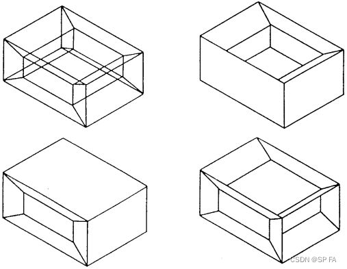
6.1.2 Surface
It generates objects with a more complete and less ambiguous representation than its wireframe model. It is obvious that surface models are suitable for more applications.
Surfaces can be 2D and 3D represented by a closed loop of curves with skin on it, the simplest form being a plane. Surfaces are built from points and curves.
They are very important in modelling objects, and in many situations, used to represent 3D models to a large variety of satisfaction.
Modelling packages usually provide a range of useful surface creation functions, some of which are similar to those for curves (but the geometric characteristics are different).
Despite their similar appearance, there are differences between surface and solid models.
Apart from the lack of volume-related information, surface models normally define the geometry of their corresponding objects. (空心的)
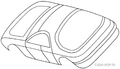
6.1.3 Solid
Solid modelling represents both the geometric properties (e.g. points, curves, surfaces, volume, centre of shape) and physical properties (e.g. mass, centre of gravity and inertia) of solid objects.
There is a number of schemes, namely primitive instancing, cell decomposition, constructive solid geometry (CSG) and boundary representation (B-Rep).
6.2 CSG
SG model is an ordered binary tree where the non-terminal nodes represent the operators and the terminal nodes are the primitives or transformation leaves.
The operators may be rigid motions or regular Boolean operations.
The primitive leaf is a primitive solid in the modelling space while the transformation leaf defines the arguments of rigid motion.
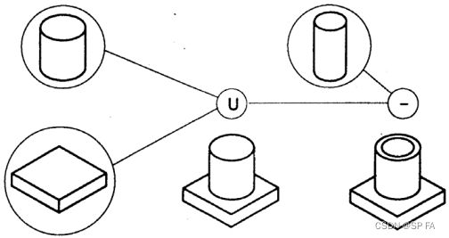
Boolean operations include Boolean Union, Boolean Difference and Boolean Intersection. It should be noticed that the resultant solid of a Boolean operation depends not only on the solids but also on their location and orientation.
Each solid usually has its local co-ordinate frame specified relative to the world co-ordinate frame.
Before a Boolean operation is performed, it may be necessary to translate and/or rotate the solids in order to obtain the required relative location and orientation relationship between them.
If an object can be represented by a unique set of data, the representation is said to be unique. The representation scheme for some applications (e.g. geometric reasoning) should ideally be both unambiguous and unique.
Solid representations are usually unambiguous but few of them can be unique, and it is not feasible to make CSG representation unique.

6.3 B-Rep
The boundary representation (B-Rep) model represents a solid by segmenting its boundary into a finite number of bounded subsets.
It is basically a topologically explicit representation. Both geometric and topological information is stored in the data structure.
The geometry is about the shape and size of the boundary entities called points, curves and surfaces while the topology keeps the connectivity of the boundary entities referred as vertices, edges and faces (corresponding to points, curves and surfaces).

The same topology may represent different geometric shapes and therefore both topological and geometric data is necessary to fully and uniquely define an object.
6.3.1 Types of B-Rep models
B-Rep models can be divided into two types: manifold and nonmanifold.
In a manifold model, an edge is connected exactly by two faces and at least three edges meet at a vertex.
A nonmanifold model may have dangling faces, edges and vertices, and therefore represent a nonrealistc object.
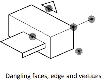
6.3.2 Euler’s law
To ensure the topological validity for a solid (i.e. manifold model), a manifold model must satisfy the following Euler (Leonhard Euler, 1707-1783) formula: V − E + F − R + 2 H = 2 S V-E+F-R+2H=2S V−E+F−R+2H=2S
where V , E , F , R , H V, E, F, R, H V,E,F,R,H and S S S are the number of vertices, edges, faces, rings (inner loops on faces), passages/holes (genus) and shells (disjoint bodies), respectively.
The Euler’s law in its simplest form is V − E + F = 2 V-E+F=2 V−E+F=2
which can be applied to simple polyhedra (i.e. objects without inner loops of edges and passages).
6.3.4 Implementation of B-Rep models
B-Rep models can be conveniently implemented on computers by representing the topology as pointers and the geometry as numerical information in the data structure for extraction and manipulation using object-oriented programming techniques.
The latest B-Rep modellers also provide facilities to tag attributes (such as colour, tolerance and surface finish) on the boundary elements.
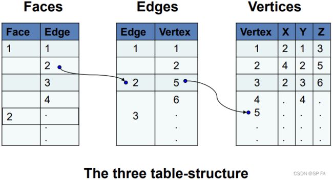
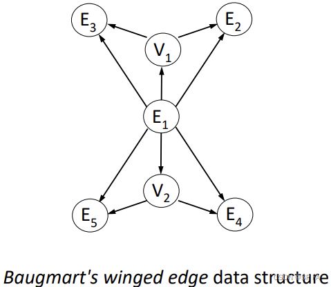
Baugmart’s winged edge data structure
a single edge, ending in two vertices, which then each has two other edges leading off from them. The edge has pointers to the vertices at its ends, and to the next edges. The vertices have pointers to their coordinates (x, y, z) and so on.
Many B-Rep modelling systems have procedures called Euler-operators. These modify the face-edge-vertex pointer structure in such a way that the Euler formula is always kept true.
An example is: make_edge_and_face(f1, v1, v3).
- This would take the cuboid on the left, and split the face into two along its diagonal, making a new object.
- Note that in the original cuboid, v1, v2, v3 and v4 must all lie in the same plane, but in the new object v2 is free to move along the top-right edge.

6.3.5 Romulus and ACIS modellers
Romulus (modeling kernel), known as Romulus (b-rep solid modeler), Romulus (disambiguation), Romulus b-rep The Romulus b-rep solid modeler (or simply Romulus) was released in 1978 by Ian Braid, Charles Lang, Alan Grayer, and the Shape Data team in Cambridge, England. It was the first commercial solid modeling kernel designed for straightforward integration into CAD software.
ACIS, known as .sab, Alan, Charles and Ian’s System (disambiguation) The 3D ACIS Modeler (ACIS) is a geometric modeling kernel developed by Spatial Corporation (formerly Spatial Technology), part of Dassault Systemes. ACIS is used by many software developers in industries such as computer-aided design (CAD), computer-aided manufacturing (CAM), computer-aided engineering (CAE), architecture, engineering and construction (AEC), coordinate-measuring machine (CMM), 3D animation and shipbuilding. ACIS provides software developers and manufacturers with the underlying 3D modeling functionality.
